TNEP model for the polarization

This tutorial demonstrates how to train a tensorial neuroevolution potential (TNEP), as presented in Xu et al. (2024). We will train a model for predicting the polarization of bulk water using the data published alongside the paper, and use the model to run molecular dynamics. For predicting the IR spectrum from a trained TNEP model, see the IR spectra tutorial.

In short, TNEP extends the NEP formalism which predicts the per-atom energies \(U_i\) as a function of atom-centered descriptors \(q_i^\gamma\),

\[U_i = U_i(q_i^\gamma).\]

We can calculate the gradients of \(U_i\) to analytically obtain the partial force \(\partial U_i / \partial r_{ij}^\nu\), where \(r_{ij}^\nu\) is the \(\nu\)-component of the interatomic distance vector \(\boldsymbol{r}_{ij} = \boldsymbol{r}_j - \boldsymbol{r}_i\). The basis for predicting tensorial properties within the TNEP framework is the partial force and the rank-2 virial tensor \(W^{\mu \nu}\), denoted as

\[W^{\mu \nu} = - \sum_i^N \sum_{j \neq i} r_{ij}^\mu \frac{\partial U_i }{\partial r_{ij}^\nu}.\]

Rank-1 tensors such as the dipole \(\mathbf{\mu}\) or the polarization \(\mathbf{P}\) might naïvely be predicted based on the partial force directly. However, this does not work as the partial forces sum to zero per construction. To circumvent this problem, the TNEP framework draws inspiration from the atomic virial, and defines rank-1 tensors based on a contraction of the rank-2 virial tensor with a vector,

\[\mathbf{P} = - \sum_i^N \sum_{j \neq i} \boldsymbol{r}_{ij} \cdot \left( \boldsymbol{r}_{ij} \otimes \frac{\partial U_i }{\partial r_{ij}} \right) = - \sum_i^N \sum_{j \neq i} r_{ij}^2 \frac{\partial U_i }{\partial r_{ij}}.\]

For rank-2 tensors such as molecular polarization \(\boldsymbol{\alpha}\) or electric susceptibility \(\boldsymbol{\chi}\), the virial tensor is slightly adapted for numerical stability,

\[\alpha^{\mu \nu} = \sum_i^N U_i \delta^{\mu \nu} - \sum_i^N \sum_{j \neq i} r_{ij}^\mu \frac{\partial U_i }{\partial r_{ij}^\nu}.\]

\(\delta^{\mu \nu}\) is the Kronecker delta, and helps stabilize the prediction of rank-2 tensor as the diagonal elements often are large than the off-diagonal elements.

Loading the dataset

We use DFT training data of polarization structures for water that are originally from Zenodo. These data are packaged together with the other files used in this tutorial notebook at Zenodo.

import os
import zipfile
import urllib.request

url = 'https://zenodo.org/records/21225618/files/tnep_polarization_training.zip'
if not os.path.exists('tnep_polarization_training'):
    urllib.request.urlretrieve(url, 'tnep_polarization_training.zip')
    with zipfile.ZipFile('tnep_polarization_training.zip') as zf:
        zf.extractall('.')
    os.remove('tnep_polarization_training.zip')
    print('Downloaded and extracted tnep_polarization_training/')
else:
    print('tnep_polarization_training/ already present')
os.chdir('tnep_polarization_training')

Downloaded and extracted tnep_polarization_training/

We load the training and test structures using ASE.

from ase.io import read

train_structures = read('train.xyz', ':')
test_structures = read('test.xyz', ':')

print(f'{len(train_structures)} structures in the training set,'
      f' and {len(test_structures)} structures in the test set.')

500 structures in the training set, and 500 structures in the test set.

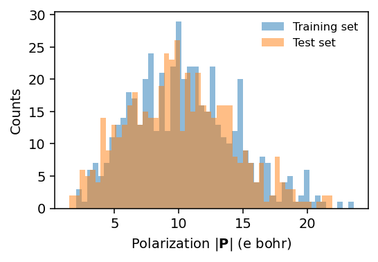
We can also inspect the polarization magnitudes:

import numpy as np

train_polarization_magnitudes = np.linalg.norm(
    [structure.get_dipole_moment() for structure in train_structures], axis=1)
test_polarization_magnitudes = np.linalg.norm(
    [structure.get_dipole_moment() for structure in test_structures], axis=1)

from matplotlib import pyplot as plt
fig, ax = plt.subplots(figsize=(4, 2.8), dpi=140)
nbins = 50
ax.hist(train_polarization_magnitudes, bins=nbins, label='Training set', alpha=0.5)
ax.hist(test_polarization_magnitudes, bins=nbins, label='Test set', alpha=0.5)
ax.set(xlabel=r'Polarization $|\mathbf{P}|$ (e bohr)', ylabel='Counts')
ax.legend(frameon=False, fontsize='small')
fig.tight_layout()

Preparing training

We can now use setup_training from calorine to prepare training of the model. The most important parameter is model_type=1, which signals to the nep executable that we aim to train a rank-1 tensorial model.

lambda_1 and lambda_2 are set to 0.0005, well below the GPUMD default of 0.05. For TNEP models the output quantities (polarization components) are typically much smaller in magnitude than energies and forces, so the default regularization strength over-regularizes the tensor outputs and leads to underfitting; smaller values are therefore recommended. For an analysis of the effect of regularization on TNEP models see Figure S13 of the Supporting Information in Xu et al. (2024). Please refer to the GPUMD documentation for details on the remaining parameters.

Some of the hyperparameters (n_max, l_max) as well as the training parameters (generation) are very generous, and the training and test sets are very large. One can achieve models with similar performance with a fraction of these, here we do not consider this aspect but rather follow the original paper.

The next cell sets up all required files for training, after which the nep executable can be launched to carry out the training.

import warnings
warnings.filterwarnings('ignore', message='Failed to retrieve stresses for structure')

from calorine.nep import setup_training

# prepare input for NEP construction
parameters = dict(version=4,
                  type=[2, 'O', 'H'],
                  model_type=1,
                  cutoff=[6, 4],
                  n_max=[6, 6],
                  basis_size=[10, 10],
                  l_max=[4, 2, 1],
                  neuron=10,
                  population=80,
                  lambda_1=0.0005,
                  lambda_2=0.0005,
                  generation=200000,
                  batch=10000)

setup_training(parameters, train_structures, rootdir='.',
               overwrite=True, mode='bagging', train_fraction=1)

Analysis of the model

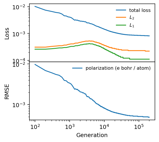
Following the completion of the training we can analyze the model performance. Here, we use the output of the reference run (rundir = 'example-output'). If you choose to run your own training, substitute your own directory below.

from calorine.nep import read_loss

rundir = 'example-output'
loss = read_loss(f'{rundir}/loss.out')

fig, axes = plt.subplots(figsize=(4, 3.6), dpi=140, nrows=2, sharex=True)

ax = axes[0]
ax.set_ylabel('Loss')
ax.plot(loss.total_loss, label='total loss')
ax.plot(loss.L2, label='$L_2$')
ax.plot(loss.L1, label='$L_1$')
ax.set_yscale('log')
ax.legend(frameon=False, fontsize='small')

ax = axes[1]
ax.plot(loss.RMSE_P_train, label='polarization (e bohr / atom)')
ax.set_xscale('log')
ax.set_yscale('log')
ax.set_xlabel('Generation')
ax.set_ylabel('RMSE')
ax.legend(frameon=False, fontsize='small')

fig.tight_layout()
fig.subplots_adjust(hspace=0, wspace=0)
fig.align_ylabels(axes)

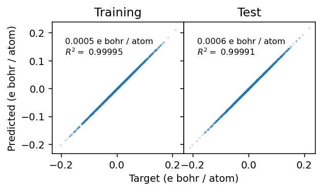
The parity plots below compare predicted and target polarization for the training and test sets. The root-mean-square error (RMSE) and coefficient of determination \(R^2\) are shown in each panel; values close to zero and one, respectively, indicate good model accuracy.

from calorine.nep import get_parity_data, read_structures

training_structures, test_structures = read_structures(rundir)
train_df = get_parity_data(training_structures, 'dipole', flatten=True)
test_df = get_parity_data(test_structures, 'dipole', flatten=True)

from sklearn.metrics import r2_score, mean_squared_error

fig, axes = plt.subplots(figsize=(4.6, 2.6), dpi=140, ncols=2,
                         sharex=True, sharey=True)

for icol, (df, label) in enumerate(zip([train_df, test_df], ['Training', 'Test'])):
    R2 = r2_score(df.target, df.predicted)
    rmse = np.sqrt(mean_squared_error(df.target, df.predicted))

    ax = axes[icol]
    ax.set_title(label)
    ax.scatter(df.target, df.predicted, alpha=0.2, s=1)
    ax.set_aspect('equal')
    ax.text(0.1, 0.75,
            f'{rmse:.4f} e bohr / atom\n' + '$R^2= $' + f' {R2:.5f}',
            transform=ax.transAxes, fontsize='small')

ax = axes[0]
ax.set_xlabel('Target (e bohr / atom)', x=1)
ax.set_ylabel('Predicted (e bohr / atom)')

fig.tight_layout()
fig.subplots_adjust(wspace=0)
fig.align_labels()

Predicting the IR spectrum

With a trained TNEP model and a PES model, an IR spectrum can be predicted from an NVE molecular dynamics trajectory. See the IR spectra tutorial for a complete walkthrough using the water model trained here.