Phonons and elastic properties

This tutorial illustrates the calculation of phonon dispersions, phonon densities of states, and the elastic stiffness tensor \(c_{ij}\), and the close relationship between them via the speed of sound.

In the first part we consider face-centered cubic (FCC) aluminum, described by NEP89, a general-purpose foundation model covering most of the periodic table, a convenient starting point since no system-specific model is required. In the second part we consider cubic BaTiO\(_3\), which, unlike aluminum, is charge-ordered: describing it with a charge-aware qNEP model rather than a plain NEP model allows us to capture the coupling between lattice vibrations and long-range electrostatics, known as LO-TO splitting, which shows up as a discontinuity in the optical phonon branches at the Brillouin zone center.

For background on crystal elasticity and the role of symmetry you can consult, e.g., Nye, Physical Properties of Crystals: Their Representation by Tensors and Matrices, Oxford University Press (1957).

The data required for running this tutorial notebook can be obtained from Zenodo.

import os
import urllib.request

os.makedirs('phonons_and_elastic_properties', exist_ok=True)
dst = 'phonons_and_elastic_properties'

# nep89.txt is a large, general-purpose model shared with other tutorials
fname = f'{dst}/nep89.txt'
if not os.path.exists(fname):
    urllib.request.urlretrieve('https://zenodo.org/records/21198312/files/nep89.txt', fname)
    print('Downloaded nep89.txt')
else:
    print('nep89.txt already present')

# The BaTiO3 NEP/qNEP pair is hosted on its own, separate Zenodo record
base_url = 'https://zenodo.org/records/18335947/files'
for fname in ['nep-BaTiO-R2SCAN.txt', 'qnep-mode2-BaTiO-R2SCAN.txt']:
    fpath = f'{dst}/{fname}'
    if not os.path.exists(fpath):
        urllib.request.urlretrieve(f'{base_url}/{fname}', fpath)
        print(f'Downloaded {fname}')
    else:
        print(f'{fname} already present')
os.chdir(dst)

Downloaded nep89.txt
Downloaded nep-BaTiO-R2SCAN.txt
Downloaded qnep-mode2-BaTiO-R2SCAN.txt

Part 1: Aluminum

Structure preparation

We start from the primitive FCC cell of aluminum and relax it using NEP89.

from ase.build import bulk
from calorine.calculators import CPUNEP
from calorine.tools import relax_structure

structure = bulk('Al')
calculator = CPUNEP('nep89.txt')
structure.calc = calculator
relax_structure(structure, fmax=0.0001)
print(f'Relaxed cell lengths: {structure.cell.lengths().round(4)} Å')

Relaxed cell lengths: [2.8213 2.8213 2.8213] Å

Compute force constants

Next we prepare the force constants from which we can obtain, for example, the phonon dispersion and the phonon density of states, using the get_force_constants() function. The third argument specifies the supercell used for computing the force constant matrix; here we use a \(3\times3\times3\) supercell. In general you need to ensure that the results are converged with respect to the supercell size.

from calorine.tools import get_force_constants

phonon = get_force_constants(structure, calculator, [3, 3, 3])

The get_force_constants function returns a Phonopy object, which provides methods for calculating various derived quantities, including the phonon dispersion and density of states.

Phonon dispersion

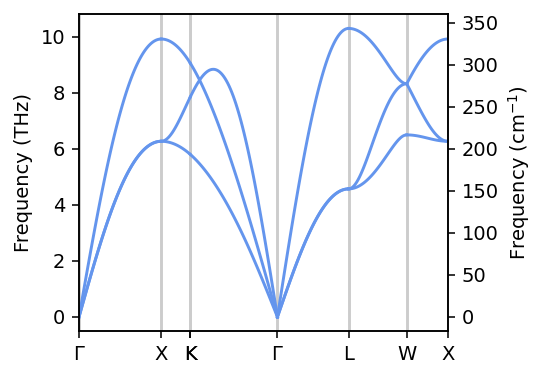
We now need to specify the path through the Brillouin zone along which the phonon dispersion is to be calculated. To this end, we use the seekpath package, which provides a standardized way for generating such paths. The \(\boldsymbol{q}\)-points returned by seekpath may refer to a different standardized primitive cell; for more information see the documentation of get_explicit_k_path.

from pandas import DataFrame
from seekpath import get_explicit_k_path

structure_tuple = (structure.cell, structure.get_scaled_positions(), structure.numbers)
path = get_explicit_k_path(structure_tuple)

phonon.run_band_structure([path['explicit_kpoints_rel']])
df = DataFrame(phonon.band_structure.frequencies[0])
df.index = path['explicit_kpoints_linearcoord']

Finally, we can plot the phonon dispersion. The most intricate task is to add the labels for the high-symmetry \(\boldsymbol{q}\)-points, which accounts for most of the lines in the next cell. We wrap this into a small helper function since we will reuse it for BaTiO\(_3\) below.

def plot_dispersion(ax, df, path, **kwargs):
    # The path may consist of several disconnected segments (e.g. a main path plus extra
    # high-symmetry lines); connecting all points with one line would draw spurious jumps
    # across segment boundaries, so each segment is plotted separately.
    for start, stop in path['explicit_segments']:
        segment = df.iloc[start:stop]
        for col in df.columns:
            ax.plot(segment.index, segment[col], **kwargs)
    ax.set_xlim(df.index.min(), df.index.max())

    labels = path['explicit_kpoints_labels']
    labels = [r'$\Gamma$' if m == 'GAMMA' else m for m in labels]
    labels = [m.replace('_', '$_') + '$' if '_' in m else m for m in labels]
    df_path = DataFrame(dict(labels=labels, positions=path['explicit_kpoints_linearcoord']))
    df_path.drop(df_path.index[df_path.labels == ''], axis=0, inplace=True)
    ax.set_xticks(df_path.positions)
    ax.set_xticklabels(df_path.labels)
    for xp in df_path.positions:
        ax.axvline(xp, color='0.8', zorder=-1)

import numpy as np
from matplotlib import pyplot as plt
from phonopy.physical_units import get_physical_units

units = get_physical_units()

fig, ax = plt.subplots(figsize=(4, 2.8), dpi=140)
plot_dispersion(ax, df, path, color='cornflowerblue')

ax.set_ylabel('Frequency (THz)')
ax2 = ax.twinx()
ax2.set_ylabel(r'Frequency (cm$^{-1}$)')
ax2.set_ylim(units.THzToCm * np.array(ax.get_ylim()))

fig.tight_layout()

Density of states

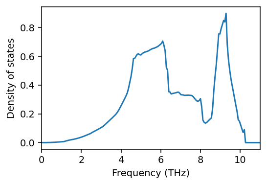
Next we compute the density of states, which requires sampling the frequencies over a mesh of \(\boldsymbol{q}\)-points that sample the Brillouin zone. This is accomplished via the run_mesh method, where the argument specifies the \(\boldsymbol{q}\)-point density.

phonon.run_mesh(30)
phonon.run_total_dos();

fig, ax = plt.subplots(figsize=(4, 2.8), dpi=140)

ax.plot(phonon.total_dos.frequency_points, phonon.total_dos.dos)
ax.set_xlabel('Frequency (THz)')
ax.set_ylabel('Density of states')
ax.set_xlim(0, 11)

fig.tight_layout()

Elastic constants and relation to sound velocities

The elastic stiffness tensor \(c_{ij}\) can be readily calculated using the get_elastic_stiffness_tensor function. The latter applies a series of deformations to the cell and fits the resulting strain energy to a Taylor expansion in strain, in which the components of the elastic stiffness tensor appear as expansion coefficients.

from calorine.tools import get_elastic_stiffness_tensor

# NEP calculator instances that have been used with get_force_constants() should not
# be reused for get_elastic_stiffness_tensor() afterward; use a fresh instance here.
structure.calc = CPUNEP('nep89.txt')
cij = get_elastic_stiffness_tensor(structure)
with np.printoptions(precision=1, suppress=True):
    print(cij)

[[113.1  65.8  65.8   0.   -0.   -0. ]
 [ 65.8 113.1  65.8  -0.    0.   -0. ]
 [ 65.8  65.8 113.1  -0.   -0.   -0. ]
 [  0.    0.   -0.   40.3   0.    0. ]
 [ -0.    0.   -0.   -0.   40.3   0. ]
 [ -0.   -0.    0.    0.    0.   40.3]]

The elastic constants are related to the sound velocity along different crystal directions. In particular \(c_{11}\) is related to the longitudinal speed of sound along \(\left<100\right>\) in the long-wavelength limit (i.e., \(\boldsymbol{q}\rightarrow 0\)) according to

\[c_s^{\left<100\right>} = \sqrt{\frac{c_{11}}{\rho}},\]

where \(\rho\) is the mass density of the material. Let us now test this relationship. For simplicity of presentation, we use the conventional 4-atom unit cell in the following, for which the cell axes are oriented along the Cartesian directions.

structure_conv = bulk('Al', cubic=True)
structure_conv.calc = calculator
relax_structure(structure_conv, fmax=0.0001)

We compute the force constants using the get_force_constants function and then use methods of the returned Phonopy object to calculate the group velocities at \(\boldsymbol{q}=(\delta, 0, 0)\) with \(\delta = 0.01\). This \(\boldsymbol{q}\)-point lies along \(\left<100\right>\) and the small \(\delta\)-value mimics the long-wavelength limit, i.e., \(\boldsymbol{q} \rightarrow 0\).

Here, the two routes agree to within about 15–20%.

from ase.units import kg

phonon_conv = get_force_constants(structure_conv, calculator, [3, 3, 3])
phonon_conv.run_band_structure([[[0.01, 0, 0]]], with_group_velocities=True)
group_velocities = np.linalg.norm(phonon_conv.band_structure.group_velocities[0], axis=2)
group_velocities *= 1e-10 / 1e-12  # Å/ps --> m/s
speed_of_sound = group_velocities[0][2]
print(f'Speed of sound, LA, <100>: {speed_of_sound:7.1f} m/s')

density = np.sum(structure_conv.get_masses()) / structure_conv.get_volume()
density /= kg * 1e-30  # amu/Å^3 --> kg/m^3
print(f'Density:                   {density:7.1f} kg/m^3')

elastic_constant = speed_of_sound ** 2 * density * 1e-9  # Pa --> GPa
print(f'Elastic constant c11:      {elastic_constant:7.1f} GPa'
      f' (direct evaluation above: {cij[0][0]:.1f} GPa)')

/home/erhart/repos/calorine/calorine/tools/phonons.py:63: PrimitiveMatrixAutoDefaultWarning: primitive_matrix defaulted to 'auto' and was resolved to a non-identity matrix:
  [-0.00000,  0.50000,  0.50000]
  [ 0.50000, -0.00000,  0.50000]
  [ 0.50000,  0.50000, -0.00000]
This differs from phonopy v3, whose default was the identity matrix. Pass primitive_matrix='P' (or --pa P on the command line) to restore the v3 behaviour.
  phonon = Phonopy(structure_ph, supercell_matrix, **kwargs_phonopy)

Speed of sound, LA, <100>:  6825.8 m/s
Density:                    2821.5 kg/m^3
Elastic constant c11:        131.5 GPa (direct evaluation above: 113.1 GPa)

Part 2: Cubic BaTiO\(_3\) (charges and the non-analytic term)

BaTiO\(_3\) is a charge-ordered perovskite: Its ions carry large, anisotropic Born effective charges (BECs), and long-range electrostatic (dipole-dipole) interactions couple to the lattice vibrations. Since capturing this coupling requires a charge-aware model, we use a qNEP model. We use a NEP/qNEP pair trained on the same R2SCAN reference data, so any difference we see below is attributable to the charge-awareness of the model rather than to differences in the training data. The models are taken from Z. Fan et al., J. Chem. Theo. Comp. 22, 4787 (2026).

Structure preparation

We build the ideal cubic perovskite structure (space group \(Pm\bar{3}m\), no. 221) directly, rather than reading it from a structure file.

from ase.spacegroup import crystal


def cubic_batio3(alat=4.0):
    return crystal(['Ba', 'Ti', 'O'], basis=[(0, 0, 0), (0.5, 0.5, 0.5), (0.5, 0.5, 0)],
                   spacegroup=221, cellpar=[alat, alat, alat, 90, 90, 90])


structure_nep = cubic_batio3()
calculator_nep = CPUNEP('nep-BaTiO-R2SCAN.txt')
structure_nep.calc = calculator_nep
relax_structure(structure_nep, fmax=1e-5)
print(f'Relaxed cell lengths: {structure_nep.cell.lengths().round(4)} Å')

Relaxed cell lengths: [4.0091 4.0091 4.0091] Å

Phonon dispersion: with and without LO-TO splitting

We now compute the phonon dispersion twice: once with the plain NEP model (no charges, no non-analytic correction), and once with the qNEP model, for which we additionally extract the BECs and the (electronic) dielectric tensor directly from the model, and feed them to phonopy as the non-analytic term (NAC) correction.

phonon_nep = get_force_constants(structure_nep, calculator_nep, [4, 4, 4])

structure_tuple = (structure_nep.cell, structure_nep.get_scaled_positions(), structure_nep.numbers)
path = get_explicit_k_path(structure_tuple)

phonon_nep.run_band_structure([path['explicit_kpoints_rel']])
df_nep = DataFrame(phonon_nep.band_structure.frequencies[0])
df_nep.index = path['explicit_kpoints_linearcoord']

For the qNEP model, get_born_effective_charges returns the BEC tensor for every atom (here flattened to shape (n_atoms, 9); we reshape it to (n_atoms, 3, 3)), and the model’s sqrt_epsilon_infinity attribute gives the (isotropic, for this cubic material) high-frequency dielectric constant.

from calorine.nep import read_model
from phonopy.interface.calculator import get_calculator_physical_units

structure_qnep = cubic_batio3()
calculator_qnep = CPUNEP('qnep-mode2-BaTiO-R2SCAN.txt')
structure_qnep.calc = calculator_qnep
relax_structure(structure_qnep, fmax=1e-5)

born_charges = calculator_qnep.get_born_effective_charges(structure_qnep).reshape(-1, 3, 3)
model = read_model('qnep-mode2-BaTiO-R2SCAN.txt')
dielectric = np.eye(3) * model.sqrt_epsilon_infinity ** 2
print(f'sqrt(epsilon_infinity) = {model.sqrt_epsilon_infinity:.3f}')

phonon_qnep = get_force_constants(structure_qnep, calculator_qnep, [4, 4, 4])
phonon_qnep.nac_params = {
    'born': born_charges,
    'factor': get_calculator_physical_units('vasp').nac_factor,
    'dielectric': dielectric,
}

phonon_qnep.run_band_structure([path['explicit_kpoints_rel']])
df_qnep = DataFrame(phonon_qnep.band_structure.frequencies[0])
df_qnep.index = path['explicit_kpoints_linearcoord']

sqrt(epsilon_infinity) = 2.799

Finally, we plot both dispersions together. Several branches are imaginary (negative frequency, plotted below the zero line). This is the well-known lattice instability of cubic BaTiO\(_3\), which drives its ferroelectric phase transition to a lower-symmetry structure at low temperature. This is thus expected and is not a model artifact; it is the reason the cubic phase does not exist as a stable structure well below the Curie temperature.

fig, ax = plt.subplots(figsize=(4, 2.8), dpi=140)
plot_dispersion(ax, df_nep, path, color='0.6', label='NEP (no charges)')
plot_dispersion(ax, df_qnep, path, color='firebrick', label='qNEP (with charges, NAC)')
ax.axhline(0, color='k', lw=0.5)
ax.set_ylabel('Frequency (THz)')

handles, labels = ax.get_legend_handles_labels()
by_label = dict(zip(labels, handles))
ax.legend(by_label.values(), by_label.keys(), frameon=False, loc='upper right', fontsize='small')

fig.tight_layout()

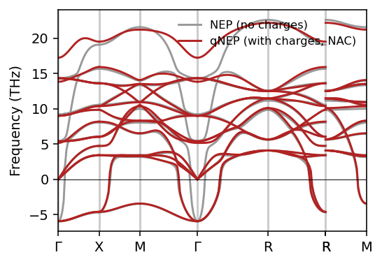
The discontinuity between the two curves at the zone center (\(\Gamma\)) for the optical branches is the LO-TO splitting: approaching \(\Gamma\) along different directions in the qNEP (charge-aware) calculation gives different limiting frequencies for the longitudinal (LO) and transverse (TO) optical modes, due to the macroscopic electric field associated with the long-range dipole-dipole interaction. The plain NEP model has no notion of atomic charges and therefore cannot reproduce this splitting at all. Its optical branches remain degenerate at \(\Gamma\).

Elastic constants: relaxed vs. clamped

In materials with internal degrees of freedom one can distinguish the so-called relaxed \(c_{ij}\) and clamped elastic constants \(c_{ij}^0\). In the former case, the ionic positions are allowed to relax after application of a macroscopic strain, whereas in the latter the relative coordinates are kept fixed. The cubic structure considered above does not feature internal degrees of freedom and therefore \(c_{ij}\) and \(c_{ij}^0\) are the same. In the tetragonal ferroelectric structure (space group \(P4mm\), no. 99) the Ti and O sublattices are, however, displaced along \(c\) relative to the ideal cubic perovskite positions, which introduces an internal degree of freedom. For demonstration we therefore consider this structure. First we create a basic version of the structure and then relax it with the qNEP model used here.

def tetragonal_batio3(alat=3.9, clat=4.1):
    return crystal(['Ba', 'Ti', 'O', 'O'], basis=[(0, 0, 0), (0.5, 0.5, 0.51), (0.5, 0.5, 0),  (0.5, 0, 0.49)],
                   spacegroup=99, cellpar=[alat, alat, clat, 90, 90, 90])


structure_tet = tetragonal_batio3()
structure_tet.calc = calculator_qnep
relax_structure(structure_tet, fmax=1e-5)
print(f'Relaxed cell lengths: {structure_tet.cell.lengths().round(4)} Å')

Relaxed cell lengths: [3.9874 3.9874 4.1221] Å

Ferroelectric perovskites are “soft” in their elastic response near the internal-coordinate relaxation direction. At the default (small) strain amplitude, the fitted relaxed constants are numerically unstable, because the harmonic small-strain expansion is ill-conditioned close to a structural instability. This is the same underlying softness already seen in the imaginary phonon branches above. Here, we therefore use a larger, still-modest strain amplitude to obtain a numerically stable fit.

structure_tet.calc = CPUNEP('qnep-mode2-BaTiO-R2SCAN.txt')
cij_rlx_tet = get_elastic_stiffness_tensor(structure_tet, fmax=1e-5, epsilon=0.02)
structure_tet.calc = CPUNEP('qnep-mode2-BaTiO-R2SCAN.txt')
cij_clamped_tet = get_elastic_stiffness_tensor(structure_tet, clamped=True, epsilon=0.02)

with np.printoptions(precision=1, suppress=True):
    print('Relaxed elastic constants')
    print(cij_rlx_tet)
    print()
    print('Clamped elastic constants')
    print(cij_clamped_tet)

Relaxed elastic constants
[[281.2 116.1  87.6   0.   -0.   -0. ]
 [116.1 281.2  87.6  -0.    0.    0. ]
 [ 87.6  87.6 125.1   0.    0.    0. ]
 [  0.   -0.    0.   54.4   0.    0. ]
 [ -0.    0.    0.    0.   52.9   0. ]
 [ -0.    0.    0.    0.    0.  109.5]]

Clamped elastic constants
[[313.2 112.4 106.    0.    0.    0. ]
 [112.4 313.2 106.    0.    0.   -0. ]
 [106.  106.  301.4   0.    0.   -0. ]
 [  0.    0.    0.  111.3   0.    0. ]
 [  0.    0.    0.    0.  111.3   0. ]
 [  0.   -0.   -0.    0.    0.  116.1]]

Unlike the cubic case, the relaxed and clamped elastic constants now differ substantially for \(c_{11}\), \(c_{33}\), and \(c_{44}\) (each 15-60% smaller when the internal coordinates are allowed to relax), while \(c_{66}\) is essentially unchanged. This pattern is consistent with symmetry: The internal degree of freedom is the Ti/O sublattice displacement along \(c\), which is the polar axis. So only strain components that couple to a \(c\)-axis atomic displacement (namely \(c_{11}\), \(c_{33}\), and the \(c\)-axis shear \(c_{44}\)) can relax against it, whereas the in-plane shear \(c_{66}\) has no such internal coordinate to couple to and is essentially unaffected.