Inspection of a NEP model

A NEP model contains a large number of parameters and hyperparameters. calorine provides functionality to parse and analyze these parameters. This is useful for obtaining insight into the model, for example, into the impact of hyperparameters but also the finer details of the descriptors and model parameters. It even consciously allows one to modify models, for example, by pruning parameters or descriptor components.

Parsing a model file and basic inspection

A model file (nep.txt) can be loaded using the read_model function, which returns a Model object that provides the content of the nep.txt in a structured format. For the following demonstration, we use a NEP4 model for cubic BaTiO\(_3\) trained against R2SCAN reference data. The model is downloaded automatically below from Zenodo, with supplementary information and other models being available here.

import os
import urllib.request

os.makedirs('nep_model_inspection', exist_ok=True)
url = 'https://zenodo.org/records/18335947/files/nep-BaTiO-R2SCAN.txt'
fname = 'nep_model_inspection/nep-BaTiO-R2SCAN.txt'
if not os.path.exists(fname):
    urllib.request.urlretrieve(url, fname)
    print('Downloaded nep-BaTiO-R2SCAN.txt')
else:
    print('nep-BaTiO-R2SCAN.txt already present')
os.chdir('nep_model_inspection')

Downloaded nep-BaTiO-R2SCAN.txt

from calorine.nep import read_model

model_fname = 'nep-BaTiO-R2SCAN.txt'
model = read_model(model_fname)

The model object behaves similarly to a dict, save for some additional functionality. It contains the basic hyperparameters of the model such as the radial and angular cutoff radii, the specifications pertaining to the basis functions for the corresponding descriptors as well as several derived quantities. A summary of its content can be obtained by using print or display (in notebooks).

display(model)

Field	Value
version	4
model_type	potential
types	('Ba', 'Ti', 'O')
radial_cutoff	6.0
angular_cutoff	4.0
n_basis_radial	8
n_basis_angular	8
n_max_radial	8
n_max_angular	6
l_max_3b	4
l_max_4b	0
l_max_5b	0
has_q_112	0
has_q_123	0
has_q_233	0
has_q_134	0
n_descriptor_radial	9
n_descriptor_angular	28
n_neuron	40
n_parameters	6014
n_descriptor_parameters	1296
n_ann_parameters	4681
sqrt_epsilon_infinity	None
charge_mode	0
restart_parameters	not available
zbl	(0.75, 1.5)
zbl_typewise_cutoff_factor	None
max_neighbors_radial	86
max_neighbors_angular	26
radial_typewise_cutoff_factor	None
angular_typewise_cutoff_factor	None
Dimension of ann_parameters	(3, 3)
Dimension of q_scaler	37
Dimension of radial_descriptor_weights	(9, 9)
Dimension of angular_descriptor_weights	(7, 9)

We can thus see immediately, for example, that this model is aware of three species (Ba, Ti, and O) and uses radial and angular cutoffs of 6 and 4 Å, respectively. The descriptor contains 9 radial and 28 angular components, and thus has a dimension of 37. The model contains 6014 parameters, which includes 4681 weights in the neural network, 1296 weights in the descriptor, and 37 parameters in the scaler. Only the neural network and descriptor weights are fit parameters. The 37 parameters of the scaler (which has the same dimension as the descriptor) are set by the standardization of the input data.

The radial descriptor weights have a dimension of \(9\times9\) for each pair of species, which corresponds to \((n_\text{max}^\text{R}+1) \times (n_\text{basis}^\text{R}+1)\). Similarly the angular descriptor weights have a dimension of \(7\times9\), corresponding to \((n_\text{max}^\text{A}+1) \times (n_\text{basis}^\text{A}+1)\). Below we will show how these weights can be used to generate a visualization of the basis functions.

Analysis of the descriptors

Radial descriptors

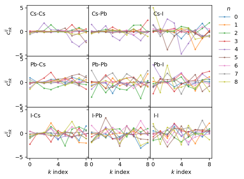
The individual fields can be accessed directly, which we can use, for example, for plotting the distribution of the weights of the descriptors. The respective fields (descriptor_weights_radial and descriptor_weights_angular) are dictionaries, where the key is a tuple containing the two species for which the weights apply. For example, we can access the weights for the Ti-O radial descriptors via potential.radial_descriptor_weights[('Ti', 'O')].

This allows us to readily plot the weights for the different combinations of species.

from matplotlib import pyplot as plt

types = model.types

fig, axes = plt.subplots(figsize=(6, 5), nrows=len(types), ncols=len(types),
                         sharex=True, sharey=True, dpi=140)

for (s1, s2), data in model.radial_descriptor_weights.items():
    irow, icol = types.index(s1), types.index(s2)
    ax = axes[irow][icol]

    for n, c_nk in enumerate(data):
        kwargs = dict(markersize=2, marker='o', alpha=0.5, label=f'{n}')
        ax.plot(c_nk, **kwargs)

    ax.set_xticks([0, 4, 8])
    if irow == len(axes) - 1:
        ax.set_xlabel('$k$ index')
    if icol == 0:
        ax.set_ylabel('$c^{ij}_{nk}$')
    ax.text(0.05, 0.8, f'{s1}-{s2}', transform=ax.transAxes)

axes[0][-1].legend(title='$n$', frameon=False,
                   loc='upper right', bbox_to_anchor=(1.5, 1.08))

fig.align_labels()
fig.subplots_adjust(hspace=0, wspace=0)

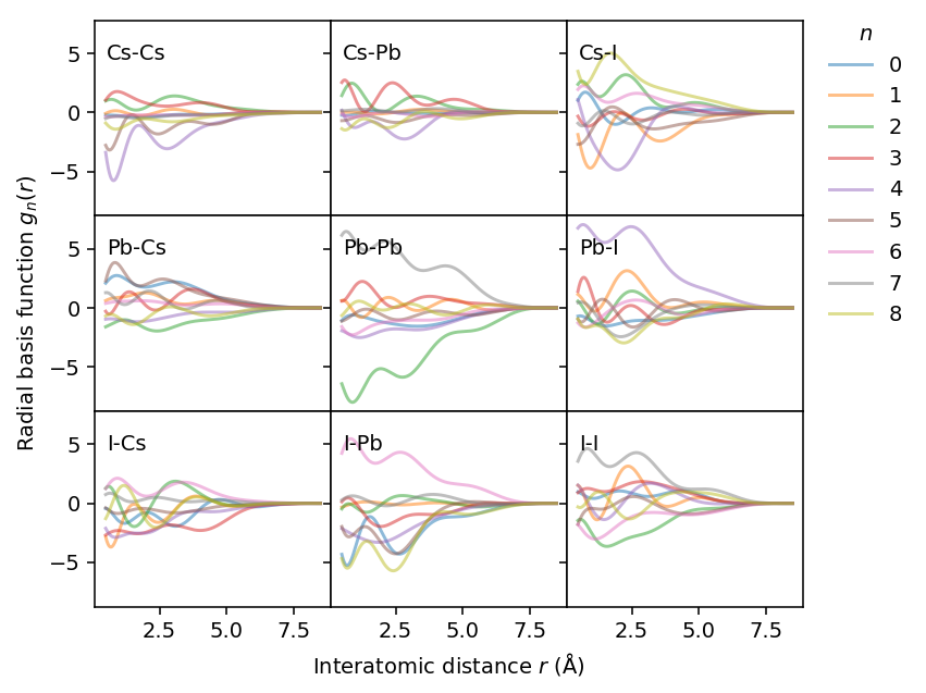
Using these weights we can also visualize the actual basis functions for the descriptor, which are obtained by adding Chebyshev polynomials.

import numpy as np
from numpy.polynomial.chebyshev import chebval


def cutoff_func(rs, rcut):
    fc = 0.5 * (1 + np.cos(np.pi * rs / rcut))
    fc[rs > rcut] = 0
    return fc

types = model.types
rs = np.arange(0.5, model.radial_cutoff + 0.5, 0.01)
xs = 2 * (rs / model.radial_cutoff - 1) ** 2 - 1

fig, axes = plt.subplots(figsize=(6, 5), nrows=len(types), ncols=len(types),
                         sharex=True, sharey=True, dpi=140)

for (s1, s2), data in model.radial_descriptor_weights.items():
    irow, icol = types.index(s1), types.index(s2)
    ax = axes[irow][icol]

    for n, c_nk in enumerate(data):
        g_n = np.zeros(len(rs))
        for k in range(len(c_nk)):
            coeff = np.zeros((k + 1))
            coeff[-1] = 1
            f_k = 0.5 * (chebval(xs, coeff) + 1) * cutoff_func(rs, model.radial_cutoff)
            g_n += c_nk[k] * f_k
        kwargs = dict(alpha=0.5, label=n)
        ax.plot(rs, g_n, **kwargs)

    if irow == len(axes) - 1 and icol == 1:
        ax.set_xlabel('Interatomic distance $r$ (Å)')
    if irow == 1 and icol == 0:
        ax.set_ylabel('Radial basis function $g_n(r)$')
    ax.text(0.05, 0.8, f'{s1}-{s2}', transform=ax.transAxes)

axes[0][-1].legend(title='$n$', frameon=False,
                   loc='upper right', bbox_to_anchor=(1.5, 1.08))

fig.align_labels()
fig.subplots_adjust(hspace=0, wspace=0)

Angular descriptors

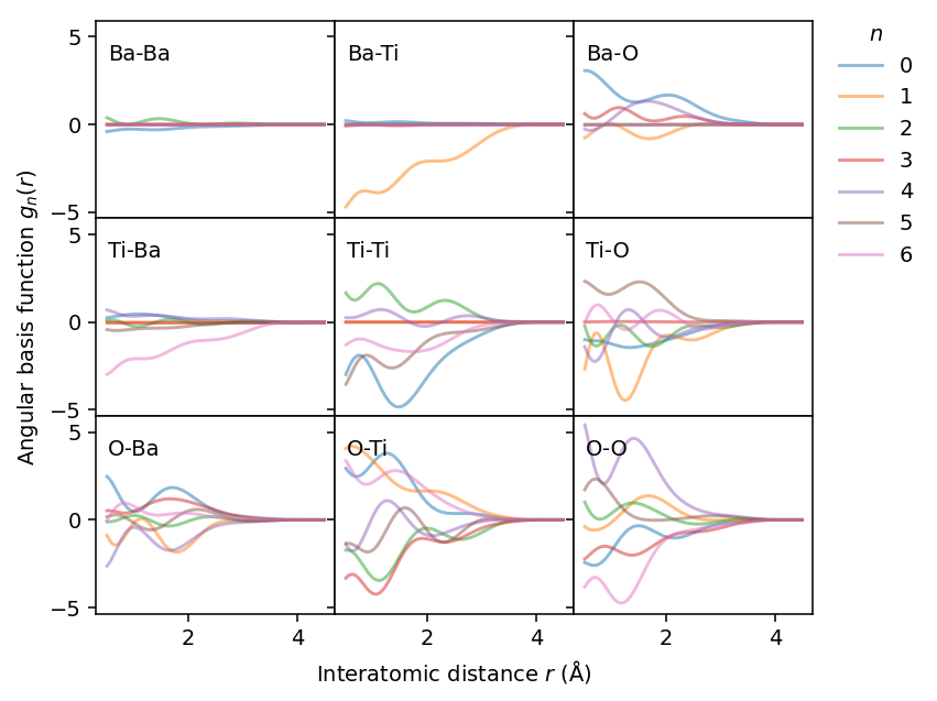
The analysis for the angular descriptor components is analogous. Here, however, the results show that angular terms are only substantial for some combinations, in particular those involving oxygen.

types = model.types
rs = np.arange(0.5, model.angular_cutoff + 0.5, 0.01)
xs = 2 * (rs / model.angular_cutoff - 1) ** 2 - 1

fig, axes = plt.subplots(figsize=(6, 5), nrows=len(types), ncols=len(types),
                         sharex=True, sharey=True, dpi=140)

for (s1, s2), data in model.angular_descriptor_weights.items():
    irow, icol = types.index(s1), types.index(s2)
    ax = axes[irow][icol]

    for n, c_nk in enumerate(data):
        g_n = np.zeros(len(rs))
        for k in range(len(c_nk)):
            coeff = np.zeros((k + 1))
            coeff[-1] = 1
            f_k = 0.5 * (chebval(xs, coeff) + 1) * cutoff_func(rs, model.angular_cutoff)
            g_n += c_nk[k] * f_k
        kwargs = dict(alpha=0.5, label=n)
        ax.plot(rs, g_n, **kwargs)

    if irow == len(axes) - 1 and icol == 1:
        ax.set_xlabel('Interatomic distance $r$ (Å)')
    if irow == 1 and icol == 0:
        ax.set_ylabel('Angular basis function $g_n(r)$')
    ax.text(0.05, 0.8, f'{s1}-{s2}', transform=ax.transAxes)

axes[0][-1].legend(title='$n$', loc='upper right',
                   bbox_to_anchor=(1.5, 1.08), frameon=False)

fig.subplots_adjust(hspace=0, wspace=0)
fig.align_labels()

Latent space representations

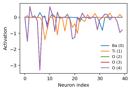
Beyond the fixed-basis-function descriptors above, we can also inspect the latent space representation of a structure: the per-atom activations of the hidden layer, obtained via get_latent_space. This is a matrix of shape (number_of_atoms, number_of_neurons), and gives a more direct view of what the network itself has learned to represent, as opposed to the fixed descriptor basis functions above.

from ase.spacegroup import crystal

from calorine.nep import get_latent_space


def cubic_batio3(alat=4.0):
    return crystal(['Ba', 'Ti', 'O'], basis=[(0, 0, 0), (0.5, 0.5, 0.5), (0.5, 0.5, 0)],
                   spacegroup=221, cellpar=[alat, alat, alat, 90, 90, 90])


structure = cubic_batio3()
latent = get_latent_space(structure, model_filename=model_fname)
print(f'Shape of latent space: {latent.shape}')

Shape of latent space: (5, 40)

fig, ax = plt.subplots(figsize=(4, 2.8), dpi=140)

for i, symbol in enumerate(structure.symbols):
    ax.plot(latent[i, :], label=f'{symbol} ({i})')
ax.set_xlabel('Neuron index')
ax.set_ylabel('Activation')
ax.legend(loc='best', frameon=False, fontsize='small')

fig.tight_layout()

Pruning a model

The model object also enables us to manipulate the model itself. One should not modify the hyperparameters such as n_max, l_max and so on, as this will lead to inconsistencies in the array dimensions and shapes. We can, however, modify the neural network (NN) or the descriptor weights. Let us now demonstrate how the model object can be used to test the effect of pruning the neural network.

The NN weights enter the model via Eq. (1) of Fan et al., Journal of Chemical Physics 157, 114801 (2022), which specifies the energy of atom \(i\) in terms of the descriptor components \(q_\nu^i\)

\[U_i = \sum_{\mu=1}^{N_\text{neu}} w_\mu^{(1)} \tanh \left( \sum_{\nu=1}^{N_\text{des}} w_{\mu\nu}^{(0)} q_{\nu}^i - b_\mu^{(0)} \right) - b^{(1)}.\]

The \(w\) and \(b\) parameters in this expression are available via the ann_parameters member in the form of a dict. Unlike NEP3 models, which share a single sub-network across all species, this NEP4 model has a separate sub-network per species. There are therefore four fields, Ba, Ti, O, and b1, where the first three each contain \(w_{\mu\nu}^{(0)}\) (→ w0), \(b_{\mu}^{(0)}\) (→ b0), and \(w_{\mu}^{(1)}\) (→ w1) for that species, while b1 contains the constant offset \(b^{(1)}\), which is shared. In the present case the descriptor has 37 components and the hidden layer contains 40 neurons, which we readily recognize in the shape of the weight arrays. Below we focus on the Ti sub-network as a representative example, since Ti off-centering is what drives the ferroelectricity of BaTiO\(_3\).

for key, value in model.ann_parameters['Ti'].items():
    print(f'{key:6} : {value.shape}')

w0     : (40, 37)
b0     : (40, 1)
w1     : (1, 40)

Let us now plot the distribution of the weights \(w_{\mu\nu}^{(0)}\) (w0) connecting the descriptor to the hidden layer on a logarithmic scale.

fig, ax = plt.subplots(figsize=(4, 2.8), dpi=140)

params = model.ann_parameters['Ti']['w0'].flatten()
_ = ax.hist(np.log10(np.abs(params)), bins=100)
ax.set_xlabel('log$_{10}$($|w_{\\mu\\nu}^{(0)}|$)')
ax.set_ylabel('Number of parameters')

fig.align_labels()
fig.tight_layout()

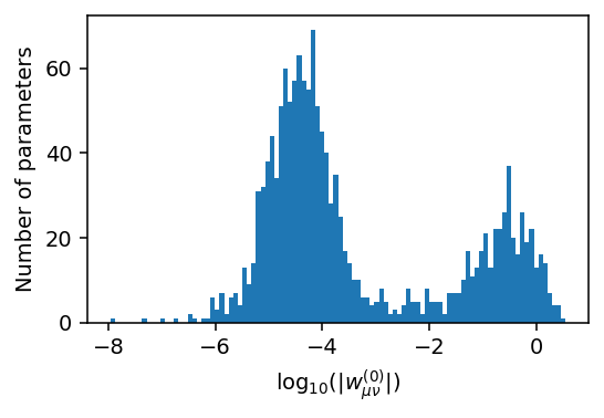
It is apparent that the majority of parameters are rather small with absolute values \(\lesssim 10^{-3}\). This distribution emerges if the optimization is run for sufficiently many generations (typically at least 100,000 generations), and is the result of the \(\ell_1\) and \(\ell_2\) regularization terms in the NEP loss function, which penalize spurious parameters.

Such a situation can occur, for example, if a particular descriptor component is not well represented by the training set, i.e., the structures in the training set only span a narrow range of values. As a result, it is difficult for the network to “learn” the impact of this particular descriptor component. If during application of the model a configuration is encountered that goes beyond this range it can lead to uncontrolled (and often unstable) behavior. Adding regularization terms combats such behavior.

Let us now remove small weights from our model to illustrate that this has (normally) a negligible effect. From the figure above, we can see that the two peaks in the distribution are separated at about \(10^{-3}\).

model_mod = read_model(model_fname)
params = model.ann_parameters['Ti']['w0']
print(f'number of non-zero parameters before pruning: {np.count_nonzero(params)}')
params = np.where(np.log10(np.abs(params)) > -3, params, 0)
print(f'number of non-zero parameters after pruning: {np.count_nonzero(params)}')
model_mod.ann_parameters['Ti']['w0'] = params
model_mod.write('nep-modified.txt')

number of non-zero parameters before pruning: 1480
number of non-zero parameters after pruning: 466

To evaluate the effect of pruning we calculate the energies of a few representative cubic BaTiO\(_3\) configurations: the relaxed structure, a uniformly strained cell, and a rattled configuration (in practice one should consider a much larger set of structures and properties).

from calorine.calculators import CPUNEP
from pandas import DataFrame

configurations = {'cubic': cubic_batio3()}

strained = cubic_batio3()
strained.set_cell(strained.cell * 1.02, scale_atoms=True)
configurations['strained'] = strained

rattled = cubic_batio3()
rattled.rattle(stdev=0.05, seed=42)
configurations['rattled'] = rattled

data = {}
for name, conf in configurations.items():
    data[name] = {}

    conf.calc = CPUNEP(model_fname)
    data[name]['original'] = conf.get_potential_energy() / len(conf)

    conf.calc = CPUNEP('nep-modified.txt')
    data[name]['pruned'] = conf.get_potential_energy() / len(conf)
df = DataFrame.from_dict(data).T
energy_shift = df.pruned.T.loc['cubic']
energy_shift -= df.original.T.loc['cubic']
print('energy cubic structure:')
print(f'  original= {df.original.T.loc["cubic"]:.5f}')
print(f'  pruned=   {df.pruned.T.loc["cubic"]:.5f} eV/atom')
print(f'  shift=    {energy_shift*1e3:.5f} meV/atom')

df.original -= df.original.T.loc['cubic']
df.pruned -= df.pruned.T.loc['cubic']
df.original *= 1e3
df.pruned *= 1e3
df['difference'] = df.pruned - df.original
df

energy cubic structure:
  original= -14.82583
  pruned=   -14.82578 eV/atom
  shift=    0.05554 meV/atom

	original	pruned	difference
cubic	0.000000	0.000000	0.000000
strained	18.657908	18.657235	-0.000673
rattled	15.833221	15.830736	-0.002485

It is apparent that the energetics are only weakly affected as the total energies only change on the order of \(10^{-5}\) eV/atom, and the energy differences between the structures differ by an even smaller amount.

Peeling the model, layer by layer

The above analysis shows that there are some connections that are effectively turned off during parameter optimization. Let us now inspect which terms these weights correspond to. Below we first plot the mean absolute weight per node in the descriptor (input) layer

\[N_\text{neu}^{-1}\sum_{\mu}^{N_\text{neu}} |w_{\mu\nu}^{(0)}|.\]

fig, ax = plt.subplots(figsize=(6, 2.8), dpi=140)

params = model.ann_parameters
nr = model.n_max_radial + 1
na = model.n_max_angular + 1
la = model.l_max_3b + model.l_max_4b + model.l_max_5b

acc_w_desc = np.mean(np.abs(params['Ti']['w0']), axis=0)
for k, w in enumerate(acc_w_desc):
    kwargs = dict()
    label, color = '', 'C0'
    if k < nr:
        if k == 0:
            label = 'radial'
    else:
        color = 'C1'
        if k == nr:
            label = 'angular'
    kwargs = dict(color=color, label=label)
    ax.bar([k], [w], **kwargs)

ax.set_xlabel('Descriptor component')
ax.set_ylabel('Mean absolute weights')
ax.legend(frameon=False, fontsize='small')

labels = [f'{r}' for r in range(nr)]
labels += [f'{n},{l}' for l in range(la) for n in range(na)]
ax.set_xticks(range(len(labels)), labels=labels, fontsize='small')

plt.xticks(rotation=90)

fig.tight_layout()

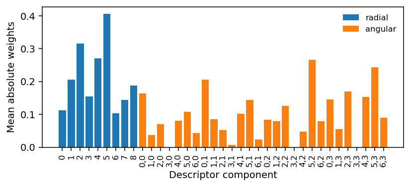
It is apparent that the radial components carry a higher overall weight in the description of the interactions than the angular components, as expected based on physical intuition. One also observes that the mean absolute weights are non-zero for all descriptor components. In other words, all of the descriptor components are active. This is different for the nodes in the hidden layer as we can see in the next figure, which shows

• the weights connecting the hidden layer to the output node \(|w_{\nu}^{(1)}|\),

• the mean absolute weight per node in the hidden layer \(N_{\mathrm{des}}^{-1} \sum_{\nu}^{N_{\mathrm{des}}} |w_{\mu\nu}^{(0)}|\) as well as

• the bias for each node in the hidden layer \(|b_{\nu}^{(0)}|\)

for the Ti sub-network.

fig, ax = plt.subplots(figsize=(4, 3.2), dpi=140)

params = model.ann_parameters
w0 = params['Ti']['w0']
w1 = params['Ti']['w1']
b0 = params['Ti']['b0']

xs = range(1, len(b0) + 1)
acc_weights = np.mean(np.abs(w0), axis=1)
ax.bar(xs, acc_weights,
       label=r'$N_{\mathrm{des}}^{-1} \sum_{\nu}^{N_{\mathrm{des}}} |w_{\mu\nu}^{(0)}|$')
abs_b0 = np.abs(b0.flatten())
ax.bar(xs, -np.abs(b0.flatten()), label=r'$|b_{\mu}^{(0)}|$ (bias)')
ax.plot(xs, w1.flatten(), 'o-', label=r'$|w_{\mu}^{(1)}|$', c='green', markersize=4)
ax.axhline(0, lw=1, c='k', alpha=0.5)

ax.set_xlabel(r'Hidden neuron index $\mu$')
ax.set_ylabel(r'Bias / Mean absolute weight')
ax.legend(frameon=False)

print('Approximate number of active neurons:', np.count_nonzero(abs_b0[abs_b0 > 0.01]))

Approximate number of active neurons: 18

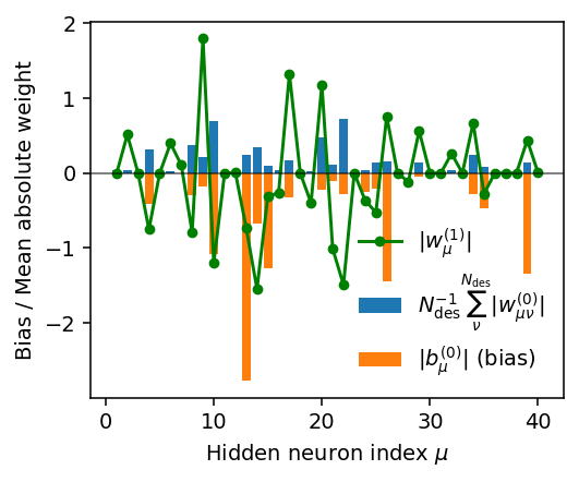
There are several neurons with very small mean absolute weight \(N_{\mathrm{des}}^{-1} \sum_{\nu}^{N_{\mathrm{des}}} |w_{\mu\nu}^{(0)}|\), implying that these neurons are effectively inactive. For the same neurons also the weights for the connections to the output node \(|w_{\mu}^{(1)}|\) as well as the bias terms \(|b_{\mu}^{(0)}|\) are small. This suggests that the number of neurons in the hidden layer could be reduced notably without a loss in accuracy, leading to faster execution.