NEP training

This tutorial demonstrates how to train a neuroevolution potential (NEP) against a set of reference calculations using calorine.nep.setup_training, and how to analyze the outcome of the training (loss curves, parity plots, parameter distributions).

We use a real density-functional-theory (DFT) reference dataset for bulk aluminum, spanning several crystal structures (fcc, bcc, hcp, diamond) both near and away from equilibrium. We train a small ensemble of models via a k-fold split of the training set (useful for estimating prediction uncertainty from the spread between ensemble members), and compare two training protocols: a straightforward single-stage run, and a two-stage curriculum that first emphasizes forces before balancing forces and energies.

Generating the reference structures themselves (prototype construction, straining, rattling, active learning, …) is not covered here; this tutorial starts from an already-assembled reference dataset.

The reference dataset

The dataset (aluminum-CX.db, an ASE database) is available on its own Zenodo record and was originally constructed for P. Ying et al., J. Chem. Phys. 162, 064109 (2025). It contains 1050 configurations of elemental aluminum with reference energies, forces, and stresses computed with VASP, covering the fcc, bcc, hcp, and diamond crystal structures, both close to and far from equilibrium (via strained, deformed, and rattled variants of each prototype as well as structures from active learning cycles).

import os
import re
import urllib.request

import ase.db

os.makedirs('nep_training', exist_ok=True)
fname = 'nep_training/aluminum-CX.db'
if not os.path.exists(fname):
    url = 'https://zenodo.org/records/13712924/files/aluminum-CX.db'
    urllib.request.urlretrieve(url, fname)
    print('Downloaded aluminum-CX.db')
else:
    print('aluminum-CX.db already present')
os.chdir('nep_training')

aluminum-CX.db already present

db = ase.db.connect('aluminum-CX.db')

structures = []
for row in db.select():
    atoms = row.toatoms()
    # the filename encodes the crystal-structure prototype, e.g.
    # 'run_fcc-alat4.000-rattled0.04-nat256-k00.xml.gz'
    name = row.get('filename', '').replace('.xml.gz', '')
    atoms.info['name'] = name
    label = re.match(r'([a-zA-Z]+)', name.replace('run_', '')).group(1)
    atoms.info['structure_type'] = label
    structures.append(atoms)

print(f'Number of structures: {len(structures)}')
print(f'Number of atoms: {sum(len(s) for s in structures)}')

Number of structures: 1050
Number of atoms: 52187

import pandas as pd

counts = pd.Series([s.info['structure_type'] for s in structures]).value_counts()
sizes = pd.Series([len(s) for s in structures])
print(counts)
print(f'Structure sizes: {sizes.min()}-{sizes.max()} atoms')

hcp        849
fcc        120
bcc         43
diamond     38
Name: count, dtype: int64
Structure sizes: 1-256 atoms

Two training protocols

calorine.nep.setup_training writes the input files (nep.in, train.xyz, test.xyz) required by the nep executable of GPUMD, given a set of parameters and a list of structures.

We request mode='kfold' with n_splits=5, which in addition to a nepmodel_full directory (all structures used for training) creates five nepmodel_split* directories, each holding a different 80%/20% train/test partition of the data. Training one model per split gives a small ensemble: the spread between the resulting predictions is a useful (if approximate) estimate of the model’s uncertainty, and comparing train/test scores per split is a convenient way to check that the model is not overfitting.

We compare two ways of training the same architecture (neuron=30, radial/angular cutoffs of 6/4 Å, l_max=[4, 2]) on the same data:

• One-stage: a single, straightforward training run for 200,000 generations with the default loss weights.

• Two-stage (curriculum) training: first train for 100,000 generations with the force term heavily up-weighted relative to the energy term (lambda_f=20, lambda_e=1), then continue for another 100,000 generations with balanced weights (lambda_f=5, lambda_e=5). The idea is that forces provide a much denser training signal per structure (3 * n_atoms values vs. a single energy value), so letting them dominate early on can help the model find a good set of descriptors before also having to fit the comparatively sparse energies well.

Both protocols use the same train/test splits (the default seed=42 in setup_training makes the k-fold partitioning deterministic), so the resulting models are directly comparable.

from calorine.nep import setup_training

shared_parameters = dict(
    version=4,
    type=[1, 'Al'],
    cutoff=[6, 4],
    l_max=[4, 2],
    neuron=30,
    batch=2000,
    save_potential=[2000, 0, 0],
)

one_stage_parameters = dict(shared_parameters, generation=200000)
setup_training(
    one_stage_parameters,
    structures,
    rootdir='nep_ensemble_one_stage',
    mode='kfold',
    n_splits=5,
    overwrite=True,
)

# the first stage of the curriculum: heavily favor forces over energies
stage1_parameters = dict(
    shared_parameters, generation=100000, lambda_f=20, lambda_e=1)
setup_training(
    stage1_parameters,
    structures,
    rootdir='nep_ensemble_two_stage',
    mode='kfold',
    n_splits=5,
    overwrite=True,
)

Running the training

Each nepmodel_* directory now contains a self-contained set of input files, and can be trained independently, e.g., as separate jobs on a cluster, by running the nep executable from within it.

For the two-stage protocol, we first need to write the second-stage nep.in (calorine.nep.write_nepfile only (re-)writes nep.in, leaving train.xyz/test.xyz untouched):

from calorine.nep import write_nepfile
from glob import glob

# balanced weights for the second stage
stage2_parameters = dict(
    shared_parameters, generation=100000, lambda_f=5, lambda_e=5)
for dname in sorted(glob('nep_ensemble_two_stage/nepmodel_*')):
    write_nepfile(stage2_parameters, dname)

and then, in each directory, run stage 1, back up its output, and restart training with the stage-2 weights. The nep executable will automatically continue from nep.restart if that file is present (see the GPUMD documentation), so all that stage 2 needs is the updated nep.in:

#!/usr/bin/env bash
# run from within a nepmodel_* directory; the stage-1/stage-2 nep.in files
# are written to the parent directory as nep-stage1.in / nep-stage2.in
cp ../nep-stage1.in nep.in
nep

mkdir stage1
cp -dr * stage1
rm -f nep_gen*.txt nep_gen*.restart   # avoid filename clashes with stage 2's checkpoints

cp ../nep-stage2.in nep.in
nep   # continues from nep.restart, which stage 1 already wrote

On a cluster, this is typically submitted as a batch job (e.g., via sbatch for SLURM), one job per nepmodel_* directory.

Note: nep.restart preserves the optimizer and model state, but not the generation counter. So after a restart, loss.out and the nep_gen*.txt checkpoints in that directory start counting from zero again, even though training is continuing from where stage 1 left off (and the same applies if a job is preempted and resubmitted, without any deliberate curriculum change). We deal with this explicitly below when combining stage 1 and stage 2 into a single, continuous view of the training history.

Downloading the example output

Training both ensembles end to end takes a while (each two-stage model, in particular, involves two full training runs), so rather than requiring you to run it before continuing with this tutorial, we provide the resulting output as a download: nep.txt, loss.out, train.xyz, test.xyz, and the nep_gen*.txt checkpoints for all ten models (five one-stage, five two-stage, plus the corresponding nepmodel_full directories). The example output is kept in separate nep_ensemble_*_example/ directories so it can never collide with your own run; the next cell uses your own nep_ensemble_*/ output if present, and otherwise downloads and uses the example.

import zipfile

one_stage_dir = 'nep_ensemble_one_stage'
two_stage_dir = 'nep_ensemble_two_stage'

if os.path.exists(f'{one_stage_dir}/nepmodel_full/loss.out'):
    print('Using your own trained nep_ensemble_*/ output')
else:
    # no real training output in nep_ensemble_*/ (setup_training() above only wrote
    # the input files); fall back to the precomputed example output instead, kept
    # under a separate _example suffix so it can never collide with your own run
    one_stage_dir = 'nep_ensemble_one_stage_example'
    two_stage_dir = 'nep_ensemble_two_stage_example'
    if not os.path.exists(f'{one_stage_dir}/nepmodel_full/loss.out'):
        url = 'https://zenodo.org/records/21198312/files/nep_training.zip'
        urllib.request.urlretrieve(url, 'nep_training.zip')
        with zipfile.ZipFile('nep_training.zip') as zf:
            zf.extractall('.')
        os.remove('nep_training.zip')
        print('Downloaded and extracted nep_ensemble_*_example/')
    else:
        print('nep_ensemble_*_example/ already present')

nep_ensemble_*_example/ already present

Analyzing the results

Loss curves

calorine.nep.read_loss reads loss.out into a DataFrame, indexed by generation in steps of 100. That index is based on row position, not on the (possibly restart-reset) step counter printed in the file itself, so we can combine the two-stage model’s stage1/loss.out with its (restarted) loss.out into one continuous history by shifting the second file’s index to start where the first one ends.

from calorine.nep import read_loss
from matplotlib import pyplot as plt

loss_one_stage = read_loss(f'{one_stage_dir}/nepmodel_full/loss.out')

loss_two_stage_stage1 = read_loss(
    f'{two_stage_dir}/nepmodel_full/stage1/loss.out')
loss_two_stage_stage2 = read_loss(
    f'{two_stage_dir}/nepmodel_full/loss.out')
stage1_end = loss_two_stage_stage1.index[-1]
loss_two_stage_stage2.index = loss_two_stage_stage2.index + stage1_end
loss_two_stage = pd.concat([loss_two_stage_stage1, loss_two_stage_stage2])

fig, axes = plt.subplots(figsize=(6, 3.4), ncols=2, sharey=True, dpi=140)

ax = axes[0]
ax.plot(loss_one_stage.RMSE_E_train, label='energy (eV/atom)')
ax.plot(loss_one_stage.RMSE_F_train, label='forces (eV/Å)')
ax.plot(loss_one_stage.RMSE_V_train, label='virial (eV/atom)')
ax.set_title('One-stage', fontsize='medium')
ax.set_xlabel('Generation')
ax.set_ylabel('Train RMSE')
ax.set_xscale('log')
ax.set_yscale('log')
ax.legend(handlelength=1, fontsize='small')

ax = axes[1]
ax.plot(loss_two_stage.RMSE_E_train, label='energy (eV/atom)')
ax.plot(loss_two_stage.RMSE_F_train, label='forces (eV/Å)')
ax.plot(loss_two_stage.RMSE_V_train, label='virial (eV/atom)')
ax.axvline(stage1_end, ls='--', color='0.5', alpha=0.7)
ax.text(stage1_end, ax.get_ylim()[1], ' stage 2 ',
        ha='left', va='top', fontsize='small')
ax.set_title('Two-stage', fontsize='medium')
ax.set_xlabel('Generation')
ax.set_xscale('log')
ax.set_xlim(1e3, 2e5)

fig.tight_layout()
fig.subplots_adjust(wspace=0)
fig.align_labels()

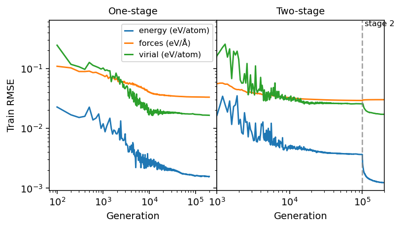
In the two-stage run the force RMSE drops faster during stage 1 (where forces are heavily up-weighted), and the energy RMSE only starts dropping appreciably once stage 2 starts at which point the weights for energies and forces are balanced, which is the intended curriculum effect.

Parity plots

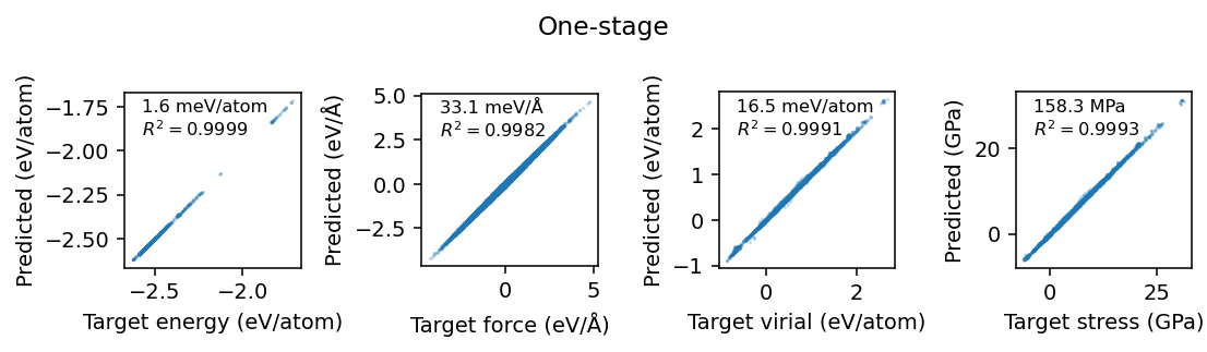
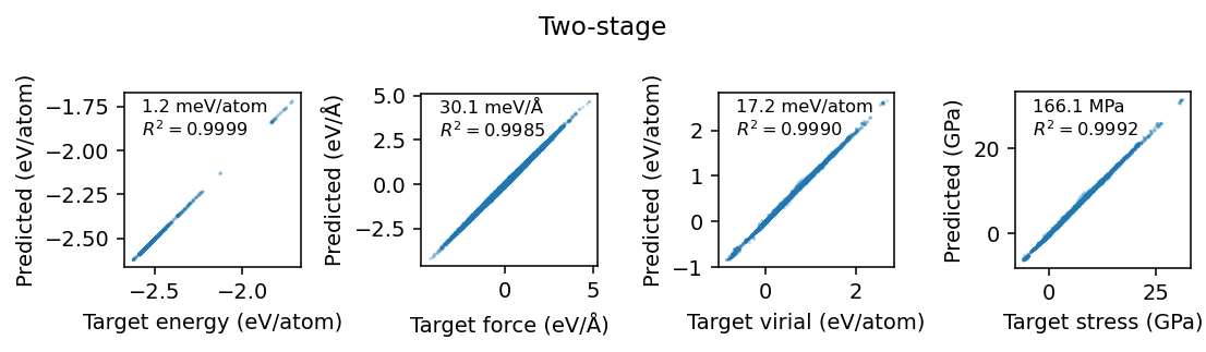
calorine.nep.read_structures reads back the structures used for training (or testing) together with the corresponding NEP predictions, and calorine.nep.get_parity_data extracts target-vs-predicted pairs for a given property. We compare the final nepmodel_full model from each protocol.

from calorine.nep import get_parity_data, read_structures
from sklearn.metrics import r2_score, root_mean_squared_error

units = dict(energy='eV/atom', force='eV/Å', virial='eV/atom', stress='GPa')

for label, dname in [
    ('One-stage', f'{one_stage_dir}/nepmodel_full'),
    ('Two-stage', f'{two_stage_dir}/nepmodel_full'),
]:

    fig, axes = plt.subplots(figsize=(8, 2.2), ncols=4, dpi=140)

    training_structures, _ = read_structures(dname)
    for ax, (prop, unit) in zip(axes, units.items()):
        df = get_parity_data(training_structures, prop, flatten=True)
        R2 = r2_score(df.target, df.predicted)
        rmse = root_mean_squared_error(df.target, df.predicted)

        ax.scatter(df.target, df.predicted, alpha=0.2, s=0.5)
        ax.set_xlabel(f'Target {prop} ({unit})')
        ax.set_ylabel(f'Predicted ({unit})')
        ax.set_aspect('equal')
        mod_unit = unit.replace('eV', 'meV').replace('GPa', 'MPa')
        ax.text(0.1, 0.75, f'{1e3*rmse:.1f} {mod_unit}\n$R^2 = ${R2:.4f}',
                fontsize='small', transform=ax.transAxes)

    fig.suptitle(label)
    fig.tight_layout()
    fig.align_labels()

Scores by crystal structure

Since the dataset spans several distinct crystal structures, it is instructive to break the energy and force errors down by prototype (recall that we stored this in structure.info['structure_type'] when we assembled the dataset).

import numpy as np

def scores_by_structure_type(training_structures):
    rows = {}
    for structure_type in sorted(set(s.info['structure_type']
                                     for s in training_structures)):
        selected = [s for s in training_structures
                    if s.info['structure_type'] == structure_type]
        row = {'N': len(selected)}
        for prop in ['energy', 'force', 'virial']:
            df = get_parity_data(selected, prop, flatten=True)
            rmse = root_mean_squared_error(df.target, df.predicted)
            row[f'RMSE_{prop}'] = np.round(1e3 * rmse, decimals=1)
        rows[structure_type] = row
    return pd.DataFrame(rows).T


print('One-stage')
training_structures, _ = read_structures(f'{one_stage_dir}/nepmodel_full')
display(scores_by_structure_type(training_structures))

print('Two-stage')
training_structures, _ = read_structures(f'{two_stage_dir}/nepmodel_full')
display(scores_by_structure_type(training_structures))

One-stage

	N	RMSE_energy	RMSE_force	RMSE_virial
bcc	43.0	2.3	27.9	11.0
diamond	38.0	0.9	31.2	12.4
fcc	120.0	3.7	35.8	23.7
hcp	849.0	0.9	31.9	15.6

Two-stage

	N	RMSE_energy	RMSE_force	RMSE_virial
bcc	43.0	1.5	23.4	14.2
diamond	38.0	0.6	25.2	8.1
fcc	120.0	2.6	32.8	20.5
hcp	849.0	0.9	29.3	17.1

Ensemble scores

For each ensemble member we can compare the RMSE on its own training and test partitions; a model that is not overfitting should show comparable train and test scores. We do this for both protocols.

def ensemble_scores(rootdir):
    rows = {}
    for dname in sorted(glob(f'{rootdir}/nepmodel_*')):
        train, test = read_structures(dname)
        row = {}
        for prop in ['energy', 'force', 'virial']:
            df = get_parity_data(train, prop, flatten=True)
            rmse = root_mean_squared_error(df.target, df.predicted)
            row[f'RMSE_{prop}_train'] = np.round(1e3 * rmse, decimals=1)
            df = get_parity_data(test, prop, flatten=True)
            rmse = root_mean_squared_error(df.target, df.predicted)
            row[f'RMSE_{prop}_test'] = np.round(1e3 * rmse, decimals=1)
        rows[dname.split('/')[-1].replace('nepmodel_', '')] = row
    return pd.DataFrame(rows).T


print('One-stage')
display(ensemble_scores(one_stage_dir))

print('Two-stage')
display(ensemble_scores(two_stage_dir))

One-stage

	RMSE_energy_train	RMSE_energy_test	RMSE_force_train	RMSE_force_test	RMSE_virial_train	RMSE_virial_test
full	1.6	1.5	33.1	36.1	16.5	26.4
split1	1.4	1.5	33.5	32.6	15.4	15.1
split2	1.6	1.5	34.4	33.4	16.0	17.0
split3	1.6	1.7	33.1	36.5	16.1	16.8
split4	1.7	1.7	34.4	33.5	16.4	15.9
split5	1.9	2.0	33.5	33.8	18.2	18.2

Two-stage

	RMSE_energy_train	RMSE_energy_test	RMSE_force_train	RMSE_force_test	RMSE_virial_train	RMSE_virial_test
full	1.2	0.2	30.1	28.6	17.2	25.2
split1	1.3	1.4	30.7	29.8	17.4	17.5
split2	1.5	1.6	30.7	29.8	19.6	20.6
split3	1.4	1.4	29.3	32.8	18.2	19.1
split4	1.3	1.4	30.3	30.2	18.3	18.3
split5	1.5	1.6	30.0	30.2	19.4	19.0

Parameter distributions

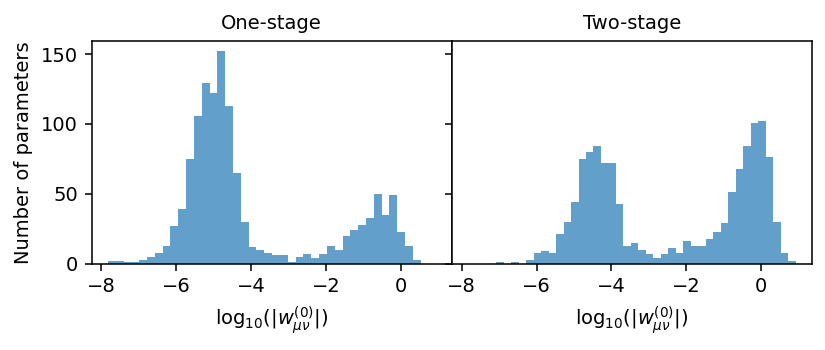
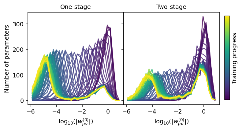
calorine.nep.read_model parses nep.txt into a Model object, which exposes the neural-network weights and biases per species via model.ann_parameters (here there is a single species, 'Al', plus the shared output bias 'b1'). Both protocols end up with a similar bimodal shape: a large population of near-zero (effectively pruned) weights plus a smaller population that meaningfully contributes, although the balance between the two populations differs somewhat between the two training paths.

from calorine.nep import read_model

fig, axes = plt.subplots(
    figsize=(6, 2.6), ncols=2, dpi=140, sharex=True, sharey=True)

for ax, (label, dname) in zip(
    axes, [('One-stage', one_stage_dir), ('Two-stage', two_stage_dir)]
):
    model = read_model(f'{dname}/nepmodel_full/nep.txt')
    params = model.ann_parameters['Al']['w0'].flatten()
    ax.hist(np.log10(np.abs(params)), bins=40, alpha=0.7)
    ax.set_title(label, fontsize='medium')
    ax.set_xlabel(r'log$_{10}(|w_{\mu\nu}^{(0)}|)$')

axes[0].set_ylabel('Number of parameters')

fig.tight_layout()
fig.subplots_adjust(wspace=0)
fig.align_labels()

Evolution during training

Since we asked setup_training to checkpoint the model every 2000 generations (save_potential=[2000, 0, 0]), we can track how the distribution of w0 weights evolves over the course of training. For the two-stage model, we again need to account for the generation counter resetting between stage1/ and the (restarted) main directory.

def checkpoint_generations(*dirs_with_offsets):
    """Yield (absolute_generation, checkpoint_path) pairs across one or more
    directories, each starting its own file-name generation count from zero
    but representing a continuation starting at the given absolute offset.
    """
    for dname, offset in dirs_with_offsets:
        files = sorted(glob(f'{dname}/nep_gen*.txt'),
                        key=lambda f: int(f.replace('.txt', '').split('gen')[-1]))
        for fname in files:
            local_generation = int(fname.replace('.txt', '').split('gen')[-1])
            yield offset + local_generation, fname


fig, axes = plt.subplots(figsize=(6, 2.8), ncols=2, dpi=140, sharey=True)
fig.subplots_adjust(right=0.87)

checkpoint_sets = {
    'One-stage': [(f'{one_stage_dir}/nepmodel_full', 0)],
    'Two-stage': [(f'{two_stage_dir}/nepmodel_full/stage1', 0),
                  (f'{two_stage_dir}/nepmodel_full', stage1_end)],
}

cmap = plt.colormaps['viridis']
for ax, (label, dirs_with_offsets) in zip(axes, checkpoint_sets.items()):
    checkpoints = list(checkpoint_generations(*dirs_with_offsets))
    for k, (generation, fname) in enumerate(checkpoints):
        m = read_model(fname)
        params = m.ann_parameters['Al']['w0'].flatten()
        hist, edges = np.histogram(np.log10(np.abs(params)), bins=30, range=(-6, 1))
        edges = edges[:-1] + 0.5 * (edges[1] - edges[0])
        ax.plot(edges, hist, color=cmap(k / max(len(checkpoints) - 1, 1)), alpha=0.8)
    ax.set_title(label, fontsize='medium')
    ax.set_xlabel(r'log$_{10}(|w_{\mu\nu}^{(0)}|)$')

axes[0].set_ylabel('Number of parameters')
sm = plt.cm.ScalarMappable(cmap=cmap, norm=plt.Normalize(0, 1))
cax = fig.add_axes((0.89, 0.15, 0.02, 0.7))

fig.colorbar(sm, cax=cax, label='Training progress', ticks=[])

fig.subplots_adjust(wspace=0)
fig.align_labels()

Next steps

The NEP models obtained in this tutorial can be used like any other NEP model, e.g., via the CPUNEP/GPUNEP calculators demonstrated in the calculator tutorial.