Descriptor space analysis#
This notebook demonstrates how to visualize the descriptor space for a collection of structures using principal component analysis (PCA) as implemented in scikit-learn.
All model required for running this tutorial notebook can be obtained from Zenodo.
[1]:
import os
import urllib.request

os.makedirs('descriptor_space_pca', exist_ok=True)
url = 'https://zenodo.org/records/22810600/files/nep-PbTe.txt'
fname = 'descriptor_space_pca/nep-PbTe.txt'
if not os.path.exists(fname):
    urllib.request.urlretrieve(url, fname)
    print('Downloaded nep-PbTe.txt')
else:
    print('nep-PbTe.txt already present')
os.chdir('descriptor_space_pca')
Downloaded nep-PbTe.txt
Set up example system and calculate descriptors#
We start by generating a few rattled structures and energy-volume (EV) curves for PbTe. The unit cell for the EV structures is repeated in order to demonstrate that not all structures in a dataset need to have the same number of atoms.
The descriptors for each structure are calculated using the calorine.nep.get_descriptors() function.
[2]:
import numpy as np
from ase.build import bulk

from calorine.nep import get_descriptors

descriptors = []
model_filename = 'nep-PbTe.txt'

# Generate a few different rattled structures
for k in range(50):
    structure = bulk('PbTe', crystalstructure='rocksalt', a=6.7)
    structure.rattle(stdev=0.2, seed=k)
    descriptors.append(get_descriptors(structure, model_filename))

# Generate a few larger structures with (rattled) energy-volume curves as well
for k in range(3):
    for volscale in np.arange(0.7, 0.85, 0.01):
        structure = bulk('PbTe', crystalstructure='rocksalt', a=6.7).repeat(2)
        latscale = volscale ** (1 / 3)
        structure.set_cell(structure.cell * latscale, scale_atoms=True)
        structure.rattle(stdev=0.2, seed=k)
        descriptors.append(get_descriptors(structure, model_filename))
Performing PCA on the descriptors#
We can now perform the PCA. The descriptors must be concatenated into a matrix with shape (total number of atoms in dataset, descriptors components).
Tip: Do not forget to check the pca.explained_variance_ratio_ property after the fit, to check if the PCA components represent the original high-dimensional descriptor space well.
[3]:
from sklearn.decomposition import PCA

# Concatenate all descriptors
all_descriptors = np.concatenate(descriptors, axis=0)
print(f'Total number of atoms in dataset: {all_descriptors.shape[0]}')
print(f'Number of descriptor components:  {all_descriptors.shape[1]}')

# Perform PCA
pca = PCA(n_components=2)
pc = pca.fit_transform(all_descriptors)

p0 = pca.explained_variance_ratio_[0]
p1 = pca.explained_variance_ratio_[1]
print(f'Explained variance for component 0: {p0:.2f}')
print(f'Explained variance for component 1: {p1:.2f}')
Total number of atoms in dataset: 868
Number of descriptor components:  30
Explained variance for component 0: 0.99
Explained variance for component 1: 0.01
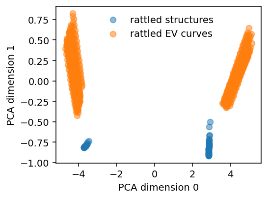
[4]:
from matplotlib import pyplot as plt

fig, ax = plt.subplots(figsize=(4, 3), dpi=140)

ax.scatter(pc[:100, 0], pc[:100, 1], alpha=0.5, label='rattled structures')
ax.scatter(pc[100:, 0], pc[100:, 1], alpha=0.5, label='rattled EV curves')
ax.set_xlabel('PCA dimension 0')
ax.set_ylabel('PCA dimension 1')
ax.legend(frameon=False)

fig.tight_layout()
Normalized vs non-normalized descriptors#
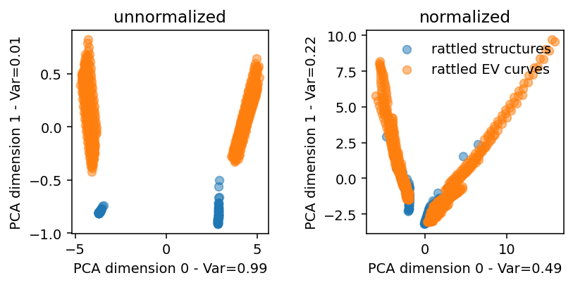
Clusters in descriptor space are often more clearly separable if the descriptors are normalized beforehand. The normalization is taken over each atom, rather than over structures. This is done in order to allow for the structures to differ in the number of atoms.
[5]:
descriptor_mean = all_descriptors.mean(axis=0)
descriptor_std = all_descriptors.std(axis=0)
normalized_descriptors = [(d - descriptor_mean) / descriptor_std for d in descriptors]
[6]:
fig, axes = plt.subplots(ncols=2, figsize=(6, 3), dpi=140)

for k, ax in enumerate(axes):
    pca = PCA(n_components=2)
    if k == 0:
        pc = pca.fit_transform(all_descriptors)
        title = 'unnormalized'
    else:
        pc = pca.fit_transform(np.concatenate(normalized_descriptors, axis=0))
        title = 'normalized'
    ax.scatter(pc[:100, 0], pc[:100, 1], alpha=0.5, label='rattled structures')
    ax.scatter(pc[100:, 0], pc[100:, 1], alpha=0.5, label='rattled EV curves')
    ax.set_xlabel(f'PCA dimension 0 - Var={pca.explained_variance_ratio_[0]:.2f}')
    ax.set_ylabel(f'PCA dimension 1 - Var={pca.explained_variance_ratio_[1]:.2f}')
    ax.set_title(title)
ax.legend(frameon=False)

fig.tight_layout()
fig.subplots_adjust(wspace=0.5)
fig.align_ylabels()