Dielectric functions

This tutorial demonstrates how to compute the dielectric function tensor \(\epsilon^{\alpha\beta}(\omega) = \epsilon_1^{\alpha\beta}(\omega) + i \epsilon_2^{\alpha\beta}(\omega)\) from a GPUMD molecular-dynamics simulation. GPUMD writes the time derivative of the polarization \(\dot{\mathbf{P}}(t)\) to a file named dpdt.out when using a qNEP model. The imaginary part of the dielectric tensor \(\epsilon_2^{\alpha\beta}(\omega)\) is related to the power spectral density of \(\dot{P}_\alpha(t)\) via

\[\epsilon_2^{\alpha\beta}(\omega) = \frac{1}{\epsilon_0 \omega V k_\mathrm{B} T}\, \mathrm{Re}\!\left[\int_0^\infty \langle \dot{P}_\alpha(0)\,\dot{P}_\beta(\tau) \rangle\, e^{-i\omega\tau}\, d\tau\right],\]

where \(V\) is the simulation cell volume, \(T\) is the temperature, and \(\epsilon_0\) is the permittivity of free space. The isotropic average \(\bar{\epsilon}_2(\omega) = \frac{1}{3}\sum_\alpha \epsilon_2^{\alpha\alpha}(\omega)\) reduces to the scalar dielectric function for cubic or isotropic systems. The real part \(\epsilon_1^{\alpha\beta}(\omega)\) is obtained component-wise via the Kramers-Kronig relation

\[\epsilon_1^{\alpha\beta}(\omega) = \frac{2}{\pi}\, \mathcal{P}\int_0^\infty \frac{\omega'\,\epsilon_2^{\alpha\beta}(\omega')}{\omega'^2 - \omega^2}\, d\omega'.\]

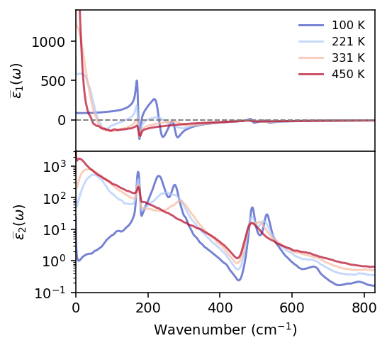
The example data are qNEP molecular-dynamics simulations of BaTiO\(_3\) at 100, 221, 331, and 450 K. These are reruns using input files similar to those of Z. Fan et al., J. Chem. Theory Comput. 22, 4787 (2026) using the same structures, but with adapted run parameters.

The data required for running this tutorial notebook can be obtained from Zenodo.

import os
import zipfile
import urllib.request

url = 'https://zenodo.org/records/22810600/files/dielectric_functions.zip'
if not os.path.exists('dielectric_functions'):
    urllib.request.urlretrieve(url, 'dielectric_functions.zip')
    with zipfile.ZipFile('dielectric_functions.zip') as zf:
        zf.extractall('.')
    os.remove('dielectric_functions.zip')
    print('Downloaded and extracted dielectric_functions/')
else:
    print('dielectric_functions/ already present')
os.chdir('dielectric_functions')

dielectric_functions/ already present

Reading the data

Each temperature has its own subdirectory (T100, T221, T331, T450) containing a 5 ns production run, with model.xyz (the simulation cell) and dpdt.out (the polarization time derivative, dumped every 20 fs). The read_dpdt function reads a dpdt.out file into a pandas.DataFrame. The columns dPx, dPy, dPz are the Cartesian components of \(\dot{\mathbf{P}}(t)\) in units of \(e\)Å/fs, and Px, Py, Pz are the corresponding polarization components in units of \(e\)Å. The time step is read directly from the time column as the difference between consecutive rows.

from ase.io import read
from calorine.gpumd import read_dpdt

temperatures = [100, 221, 331, 450]  # K

dfs_raw = {T: read_dpdt(f'T{T}/dpdt.out') for T in temperatures}
volumes = {T: read(f'T{T}/model.xyz').get_volume() for T in temperatures}

for T in temperatures:
    print(f'{T:4} K: volume = {volumes[T]:.1f} Angstrom^3, {len(dfs_raw[T])} frames')

dfs_raw[450].head()

 100 K: volume = 527788.9 Angstrom^3, 250000 frames
 221 K: volume = 529222.8 Angstrom^3, 250000 frames
 331 K: volume = 530789.4 Angstrom^3, 250000 frames
 450 K: volume = 531196.7 Angstrom^3, 250000 frames

	time	dPx	dPy	dPz	Px	Py	Pz
0	0.02	-1.926350	-4.03456	-0.377649	-38.5271	-80.69120	-7.55298
1	0.04	0.434974	-1.83067	-0.611361	-29.8276	-117.30500	-19.78020
2	0.06	0.117376	1.55974	-0.388794	-27.4801	-86.10990	-27.55610
3	0.08	-2.777010	4.71552	0.811376	-83.0202	8.20046	-11.32860
4	0.10	0.286943	5.17358	-1.085420	-77.2814	111.67200	-33.03690

Computing the dielectric function

get_dielectric_function computes both parts of the dielectric tensor from all three Cartesian components of \(\dot{\mathbf{P}}(t)\), returning the six unique Voigt components of the imaginary part \(\epsilon_2^{\alpha\beta}(\omega)\) together with the real part \(\epsilon_1^{\alpha\beta}(\omega)\) obtained via the Kramers-Kronig relation. The required physical parameters are

• volume: the simulation cell volume in Å\(^3\),

• temperature: the temperature in K.

The keyword column='dP' (the default) selects the dPx/dPy/dPz columns from read_dpdt. The time step is extracted automatically from the time column. The optional parameter t_sigma sets the width of a Gaussian window applied to the autocorrelation function before the Fourier transform (in ps); smaller values produce smoother spectra while larger values yield sharper features. window_size sets how much of the autocorrelation function (in ps, the same unit as t_sigma) is kept before the Fourier transform. If left unset, it defaults to 5 * t_sigma when t_sigma is given, or to the full trajectory otherwise.

A performance note: window_size directly sets the size of the frequency grid handed to the Kramers-Kronig step, and the default kk_method='vectorized' scales as \(\mathcal{O}(n^2)\) in both time and memory. With our 5 ns/250,000-frame runs, leaving window_size unset together with t_sigma=2 ps would already give a modest ~10,000-point grid (5 * t_sigma), but a longer t_sigma or an explicit large window_size can easily produce a grid whose vectorized Kramers-Kronig step would need tens of gigabytes. get_dielectric_function estimates this upfront and raises a clear error (governed by kk_max_memory_gb, default 4 GB) rather than letting the process hang or get killed due to an out-of-memory (OOM) error. Since the t_sigma=2 ps Gaussian window already damps the autocorrelation function well within a much shorter lag, we explicitly pass a window_size=100 ps window below (rather than relying on the 5 * t_sigma = 10 ps default) to be conservative. This gives a visually identical spectrum to a much larger window while keeping the computation fast and memory-friendly. We are, however, still benefiting from the oversampling of a long trajectory; see section on convergence with run length below.

%%time
from calorine.tools import get_dielectric_function

t_sigma = 2  # Gaussian window width in ps; smaller values give smoother spectra
window_size = 100  # ps; see note above on why this is larger than the 5*t_sigma default

dfs = {}
for T in temperatures:
    dfs[T] = get_dielectric_function(
        dfs_raw[T], volumes[T], T, column='dP', t_sigma=t_sigma, window_size=window_size)
dfs[450].head()

CPU times: user 12.1 s, sys: 5.27 s, total: 17.4 s
Wall time: 17.4 s

	angular_frequency	wavenumber_invcm	epsilon_imag_xx	epsilon_imag_yy	epsilon_imag_zz	epsilon_imag_yz	epsilon_imag_xz	epsilon_imag_xy	conductivity_xx	conductivity_yy	conductivity_zz	conductivity_yz	conductivity_xz	conductivity_xy	epsilon_real_xx	epsilon_real_yy	epsilon_real_zz	epsilon_real_yz	epsilon_real_xz	epsilon_real_xy
0	0.031419	0.166799	11427.003739	5386.194993	4200.869050	-583.749950	-229.460399	731.082956	3178.881976	1498.387379	1168.641160	-162.393593	-63.833665	203.380211	7131.346872	3914.360129	3235.856750	-313.418243	-131.080433	378.598390
1	0.062838	0.333597	5760.691497	2720.451643	2123.505602	-293.583576	-115.190481	366.982162	3205.137372	1513.606697	1181.477461	-163.344226	-64.089756	204.181780	4261.499341	2562.983119	2182.255631	-166.648484	-73.347444	194.639373
2	0.094257	0.500396	3892.771476	1844.002242	1441.282901	-197.613841	-77.301088	246.246085	3248.794180	1538.950793	1202.852911	-164.922781	-64.513247	205.509841	2745.416205	1848.803577	1625.265554	-89.175421	-42.901213	97.616953
3	0.125676	0.667195	2974.312746	1414.847436	1107.820545	-150.185491	-58.502424	186.340708	3309.700214	1574.387518	1232.739865	-167.120607	-65.099235	207.352735	2265.095597	1622.770305	1448.924603	-64.637685	-33.275813	66.924750
4	0.157095	0.833994	2435.486917	1164.578111	913.834414	-122.165131	-47.335252	150.756117	3387.644583	1619.871863	1271.099500	-169.925793	-65.841047	209.694472	2047.067926	1520.402042	1368.997336	-53.508331	-28.930168	53.045736

Kramers-Kronig integration method

The Kramers-Kronig step is performed internally by get_dielectric_function (controlled by return_real_part, which defaults to True). Two integration methods are available via the kk_method keyword:

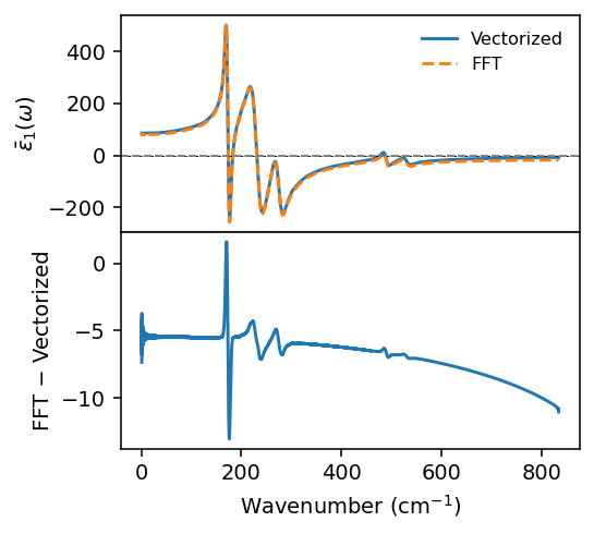
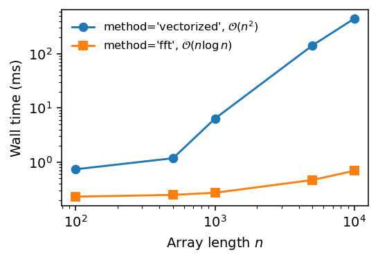
• 'vectorized' (default): exact trapezoid rule, \(\mathcal{O}(n^2)\) time and memory.

• 'fft': \(\mathcal{O}(n \log n)\) Hilbert-transform approximation; faster for large arrays but can deviate near sharp features.

The section below compares both methods on the 100 K data, which has the sharpest phonon peaks and provides the most stringent test.

Visualization

from matplotlib import pyplot as plt

def isotropic_average(df, prefix):
    return (df[f'{prefix}_xx'] + df[f'{prefix}_yy'] + df[f'{prefix}_zz']) / 3


fig, (ax1, ax2) = plt.subplots(2, 1, figsize=(4, 3.6), dpi=140, sharex=True)

cmap = plt.colormaps['coolwarm']
for T in temperatures:
    df = dfs[T]
    kwargs = dict(label=f'{T} K', color=cmap((T - 100) / (450 - 100)), alpha=0.7)
    ax1.plot(df.wavenumber_invcm, isotropic_average(df, 'epsilon_real'), **kwargs)
    ax2.plot(df.wavenumber_invcm, isotropic_average(df, 'epsilon_imag'), **kwargs)

ax1.axhline(0, color='0.5', linewidth=1, linestyle='--')
ax1.set_ylabel(r'$\widebar{\epsilon}_1(\omega)$')
ax1.legend(frameon=False, fontsize='small')
ax1.set_xlim(0, 830)
ax1.set_ylim(-400, 1400)

ax2.set_xlabel(r'Wavenumber (cm$^{-1}$)')
ax2.set_ylabel(r'$\widebar{\epsilon}_2(\omega)$')
ax2.set_yscale('log')
ax2.set_ylim(0.1, 3e3)

fig.tight_layout()
fig.subplots_adjust(hspace=0)

Convergence with run length

Each of the runs above is 5 ns long, which allows substantial oversampling and thus reduces numerical noise by better statistics. To see how much this matters, we recompute the spectrum for one temperature (331 K) using only the first 0.1, 0.2, 0.5, 1, or 5 ns of the same trajectory; get_dielectric_function takes the time series DataFrame directly, so a shorter “run” is a row-count truncation of it. To isolate the effect of run length from the choice of autocorrelation window, we keep the window itself fixed at 50 ps for every truncation; since window_size is now an absolute time in ps rather than a fraction of the trajectory length, this requires no rescaling. What changes between curves is thus purely how much data went into estimating the autocorrelation function at each lag, not the frequency resolution.

T_conv = 331
lengths_ns = [0.1, 0.2, 0.5, 1, 5]
window_ps = 50  # fixed autocorrelation window, independent of run length

fig, ax = plt.subplots(figsize=(4, 2.8), dpi=140)

cmap = plt.colormaps['viridis']
for k, length_ns in enumerate(lengths_ns):
    df = dfs_raw[T_conv]
    df = df[df.time <= 1e3 * length_ns]
    actual_length_ns = df.time.max() / 1e3
    result = get_dielectric_function(
        df, volumes[T_conv], T_conv, column='dP',
        t_sigma=t_sigma, window_size=window_ps, return_real_part=False)
    ax.plot(result.wavenumber_invcm, isotropic_average(result, 'epsilon_imag'),
            color=cmap(k / (len(lengths_ns) - 1)), label=f'{actual_length_ns} ns')

ax.set_xlabel(r'Wavenumber (cm$^{-1}$)')
ax.set_ylabel(r'$\widebar{\epsilon}_2(\omega)$')
ax.set_yscale('log')
ax.set_xlim(0, 830)
ax.legend(title='Run length', frameon=False, fontsize='small', title_fontsize='small')

fig.tight_layout()

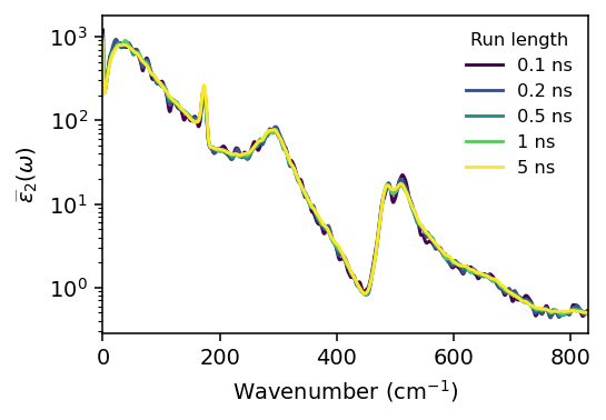
The overall shape is already recognizable from just 0.1 ns, but the shorter runs are visibly noisier. Longer trajectories average over more statistically independent time origins, giving a smoother, more reliable estimate of the autocorrelation function at each lag. 5 ns is comfortably enough to suppress this noise for this system.

Accuracy: FFT vs. vectorized

dfs[100] was computed with the default kk_method='vectorized'. The next cell below recomputes the 100 K spectrum with kk_method='fft' for comparison. The two methods agree well across most of the spectrum, but the FFT approximation can deviate near sharp features and at larger frequencies.

%%time

df_vec = dfs[100].iloc[5:]
df_fft = get_dielectric_function(dfs_raw[100], volumes[100], 100, column='dP',
                                 t_sigma=t_sigma, window_size=window_size, kk_method='fft').iloc[5:]

CPU times: user 418 ms, sys: 21.9 ms, total: 440 ms
Wall time: 439 ms

fig, (ax1, ax2) = plt.subplots(2, 1, figsize=(4, 3.6), dpi=140, sharex=True)

ax1.plot(df_vec.wavenumber_invcm, isotropic_average(df_vec, 'epsilon_real'), label='Vectorized')
ax1.plot(df_fft.wavenumber_invcm, isotropic_average(df_fft, 'epsilon_real'), '--', label='FFT')
ax1.axhline(0, color='k', linewidth=0.5, linestyle='--')
ax1.set_ylabel(r'$\bar{\epsilon}_1(\omega)$')
ax1.legend(frameon=False, fontsize='small')

diff = isotropic_average(df_fft, 'epsilon_real').to_numpy() - isotropic_average(df_vec, 'epsilon_real').to_numpy()
ax2.plot(df_vec.wavenumber_invcm, diff)
ax1.axhline(0, color='0.5', linewidth=1, linestyle='--')
ax2.set_xlabel(r'Wavenumber (cm$^{-1}$)')
ax2.set_ylabel('FFT − Vectorized')

fig.tight_layout()
fig.subplots_adjust(hspace=0)

Kramers-Kronig performance

The timing comparison below illustrates the performance advantage of the 'fft' method over the 'vectorized' approach, which comes at a small cost in accuracy (see above).

%%time

from calorine.tools import apply_kramers_kronig
import time
import numpy as np
from pandas import DataFrame

sizes = [100, 500, 1000, 5000, 10000]
times_vec = []
times_fft = []

for n in sizes:
    df_test = DataFrame({'angular_frequency': np.linspace(0.1, 100.0, n),
                         'epsilon_imag': np.sin(np.linspace(0.1, 100.0, n))})

    nrep = max(3, 200 // n)
    t0 = time.perf_counter()
    for _ in range(nrep):
        apply_kramers_kronig(df_test, method='vectorized')
    times_vec.append((time.perf_counter() - t0) / nrep * 1000)

    t0 = time.perf_counter()
    for _ in range(500):
        apply_kramers_kronig(df_test, method='fft')
    times_fft.append((time.perf_counter() - t0) / 500 * 1000)

CPU times: user 5.86 s, sys: 15.2 s, total: 21 s
Wall time: 21 s

fig, ax = plt.subplots(figsize=(4, 2.8), dpi=140)
ax.loglog(sizes, times_vec, 'o-', label=r"method='vectorized', $\mathcal{O}(n^2)$")
ax.loglog(sizes, times_fft, 's-', label=r"method='fft', $\mathcal{O}(n \log n)$")
ax.set_xlabel('Array length $n$')
ax.set_ylabel('Wall time (ms)')
ax.legend(frameon=False, fontsize='small')
fig.tight_layout()

Refractive index and absorption coefficient

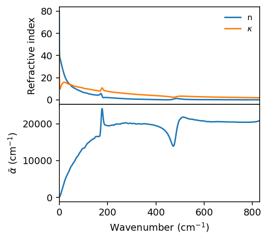
The complex dielectric function can be converted into the complex index of refraction \(N(\omega) = n(\omega) + i\kappa(\omega)\) via get_refractive_index, and the extinction coefficient \(\kappa(\omega)\) into the absorption coefficient \(\alpha(\omega)\) (in cm\(^{-1}\)) via get_absorption_coefficient. Both functions operate component-wise on the same Voigt-labeled columns produced by get_dielectric_function, so they can be chained directly onto its output. The inverse conversion, from \(n,\kappa\) (or \(n,\alpha\)) back to \(\epsilon_1,\epsilon_2\), is available via get_dielectric_function_from_refractive_index.

from calorine.tools import get_refractive_index, get_absorption_coefficient

df_nk = get_refractive_index(dfs[450])
df_nk = get_absorption_coefficient(df_nk)

fig, (ax1, ax2) = plt.subplots(2, 1, figsize=(4, 3.6), dpi=140, sharex=True)

ax1.plot(df_nk.wavenumber_invcm, isotropic_average(df_nk, 'refractive_index_real'), label='n')
ax1.plot(df_nk.wavenumber_invcm, isotropic_average(df_nk, 'refractive_index_imag'), label=r'$\kappa$')
ax1.legend(frameon=False, fontsize='small')
ax1.set_ylabel('Refractive index')
ax1.set_xlim(0, 830)

ax2.plot(df_nk.wavenumber_invcm, isotropic_average(df_nk, 'absorption_coefficient'))
ax2.set_xlabel(r'Wavenumber (cm$^{-1}$)')
ax2.set_ylabel(r'$\bar\alpha$ (cm$^{-1}$)')

fig.tight_layout()
fig.subplots_adjust(hspace=0)