
Raman spectra#
Introduction#
Raman spectroscopy probes vibrational modes that modulate the electric susceptibility \(\boldsymbol{\chi}\) of a material. The Raman intensity is proportional to the power spectral density of the time derivative of \(\boldsymbol{\chi}(t)\), evaluated along a molecular dynamics trajectory.
First-order Raman scattering involves a single phonon and is governed by crystal symmetry selection rules. BaZrO\(_3\) in its cubic phase (space group Pm\(\bar{3}\)m) is inactive for first-order Raman scattering; only second-order (two-phonon) scattering is allowed. Under pressure, BaZrO\(_3\) undergoes a cubic-to-tetragonal phase transition, which the NEP model used here predicts to occur at approximately 14 to 16 GPa. In the tetragonal phase, first-order Raman becomes allowed and produces peaks that are considerably more intense than the second-order features.
TNEP models provide the susceptibility \(\boldsymbol{\chi}(t)\) at each MD step. get_raman_spectrum converts the autocorrelation function of \(\boldsymbol{\chi}(t)\) to the Raman spectrum. See the TNEP susceptibility tutorial for how to train the susceptibility model used here, and the TNEP polarization tutorial for the rank-1 (polarization) variant.
This tutorial is based on the work of Rosander et al., Phys. Rev. B 111, 064107 (2025) and Fransson et al., Chem. Mater. 36, 514 (2024). The TNEP formalism is described in Xu et al., J. Chem. Theory Comput. 20, 3273 (2024).
Simulation setup#
The simulations use a 20×20×20 supercell of the 5-atom cubic BaZrO\(_3\) primitive cell (40,000 atoms) and two NEP models:
nep_energy.txt: the PES (potential energy surface) model (NEP4).nep_susceptibility.txt: the rank-2 TNEP susceptibility model, identical to the model trained in the TNEP susceptibility tutorial.
The simulation protocol is:
NPT equilibration: 50,000 steps × 2 fs = 100 ps at 300 K and target pressure, using the stochastic cell-rescaling (SCR) barostat.
NVE production: 500,000 steps × 2 fs = 1 ns;
dump_polarizability 5writes \(\boldsymbol{\chi}(t)\) every 5 × 2 fs = 10 fs, giving 100,000 frames per run.
Simulations are run at pressures from 0 to 20 GPa to span the cubic-to-tetragonal phase transition. Each run takes approximately 30 minutes on a single NVIDIA GH200 GPU. Using the above settings you can run the MD yourself, but you can also download the pre-computed trajectories from Zenodo by running the next cell.
[1]:
import os
import zipfile
import urllib.request

url = 'https://zenodo.org/records/22810600/files/raman_spectra.zip'
if not os.path.exists('raman_spectra'):
    urllib.request.urlretrieve(url, 'raman_spectra.zip')
    with zipfile.ZipFile('raman_spectra.zip') as zf:
        zf.extractall('.')
    os.remove('raman_spectra.zip')
    print('Downloaded and extracted raman_spectra/')
else:
    print('raman_spectra/ already present')
os.chdir('raman_spectra')
Downloaded and extracted raman_spectra/
[2]:
from ase.io import read

basedir = '.'
atoms = read(f'{basedir}/300K-0GPa/model.xyz')
natoms = len(atoms)
print(f'{natoms} atoms ({natoms // 5} formula units BaZrO3)')
print(f'Cell: {atoms.cell.lengths().round(3)} Å')
40000 atoms (8000 formula units BaZrO3)
Cell: [84.18  84.174 84.196] Å
Raman spectrum at 300 K, 0 GPa#
We start with the cubic phase at ambient pressure. As BaZrO\(_3\) is Raman inactive in first order at 0 GPa, the spectrum is dominated by second-order (two-phonon) scattering.
The accessible frequency range is bounded at both ends. The lower cutoff is set by the Gaussian window t_sigma: it broadens spectral lines to \(\sigma_{\tilde{\nu}} = 1/(2\pi c\,t_\sigma) \approx 5\,\mathrm{cm}^{-1}\) (FWHM \(\approx\) 12 cm\(^{-1}\)) for t_sigma = 1 ps, so features below approximately 25 cm\(^{-1}\) are not reliably resolved. window_size (how much of the ACF is kept before the Fourier transform) defaults to \(5\,t_\sigma\), which already
gives a frequency grid spacing \(\Delta\tilde{\nu} \approx 0.6\,\sigma_{\tilde{\nu}}\), finer than the broadening itself, so the default requires no adjustment for resolution. Because this default no longer scales with the NVE run length, running longer does not by itself sharpen this cutoff; only reducing t_sigma does, provided the run is long enough to keep the autocorrelation function well-converged out to \(5\,t_\sigma\). The upper cutoff follows from the Nyquist criterion:
\(\tilde{\nu}_\mathrm{max} = 1/(2\,c\,\Delta t)\) where \(\Delta t = 10\) fs gives \(\tilde{\nu}_\mathrm{max} \approx 1667\,\mathrm{cm}^{-1}\), well above the BaZrO\(_3\) Raman features.
GPUMD writes the total susceptibility of the cell. normalize=True divides the six components by the atom count on the num_atoms line of the polarizability.out header. That count has to match the scale the TNEP model was trained against; pass scale where it does not.
[3]:
from calorine.gpumd import read_polarizability
from calorine.tools import get_raman_spectrum

folder = f'{basedir}/300K-0GPa'
chi_df = read_polarizability(f'{folder}/polarizability.out', normalize=True)

raman_df = get_raman_spectrum(
    chi_df, t_sigma=1.0,
    polarization_in=[1, 0, 0], polarization_out=[1, 0, 0])
raman_df.head()
[3]:
| angular_frequency | wavenumber_invcm | raman_isotropic | raman_anisotropic | raman_polarized | |
|---|---|---|---|---|---|
| 0 | 0.000000 | 0.00000 | 2.696604e-20 | 8.806972e-20 | 4.080035e-20 |
| 1 | 0.628947 | 3.33898 | 2.427358e-20 | 8.261583e-20 | 3.710181e-20 |
| 2 | 1.257895 | 6.67796 | 1.811690e-20 | 6.957210e-20 | 2.855130e-20 |
| 3 | 1.886842 | 10.01694 | 1.202083e-20 | 5.536789e-20 | 1.991183e-20 |
| 4 | 2.515790 | 13.35592 | 7.813873e-21 | 4.409141e-20 | 1.378987e-20 |
Quantum corrections for second-order Raman#
Classical MD samples the Boltzmann distribution and underestimates spectral intensities at frequencies where \(\hbar\omega \gtrsim k_\mathrm{B}T\). For second-order scattering, the correction depends on the type of two-phonon process:
Overtone: two identical phonons each at \(\omega/2\):
\[f_\mathrm{ot}(\omega) = \left[\frac{\beta\hbar\omega/2}{1-e^{-\beta\hbar\omega/2}}\right]^2 \!\!(2 - e^{-\beta\hbar\omega/2})\]Combination band: two different phonons summing to \(\omega\):
\[f_\mathrm{cb}(\omega) = \left[\frac{\beta\hbar\omega/2}{1-e^{-\beta\hbar\omega/2}}\right]^2\]
These are applied via apply_quantum_correction with order='overtone' and order='combination'. First-order Raman (tetragonal phase) uses order='first' (standard single-phonon Bose-Einstein factor).
[4]:
from pandas import read_json
from calorine.tools import apply_quantum_correction

temperature = 300  # K

raman_cb = apply_quantum_correction(
    raman_df, temperature, 'raman_polarized', order='combination')

wn = raman_df['wavenumber_invcm']
mask_700 = (wn > 600) & (wn < 800)
norm_factor = raman_cb['raman_polarized_qm'][mask_700].max()


def norm(s):
    return s / norm_factor


# Experimental data (Toulouse et al., Phys. Rev. B 100, 134102 (2019))
expt = read_json(f'{basedir}/experimental-data-Toulouse2019-fig2b.json')
[5]:
from matplotlib import pyplot as plt

fig, ax = plt.subplots(figsize=(4, 3.2), dpi=140)

ax.plot(wn, norm(raman_df['raman_polarized']), label='classical')
ax.plot(wn, norm(raman_cb['raman_polarized_qm']),
        label='combination correction')
ax.plot(expt['frequency'], expt['intensity'],
        'k--', label='expt. Z(XX)Z (Toulouse 2019)')
ax.set_xlabel(r'Wavenumber (cm$^{-1}$)')
ax.set_ylabel('Z(XX)Z Raman intensity (normalized)')
ax.set_xlim(50, 1400)
ax.set_ylim(0, 1.35)
ax.legend(frameon=False, fontsize='small')

fig.tight_layout()
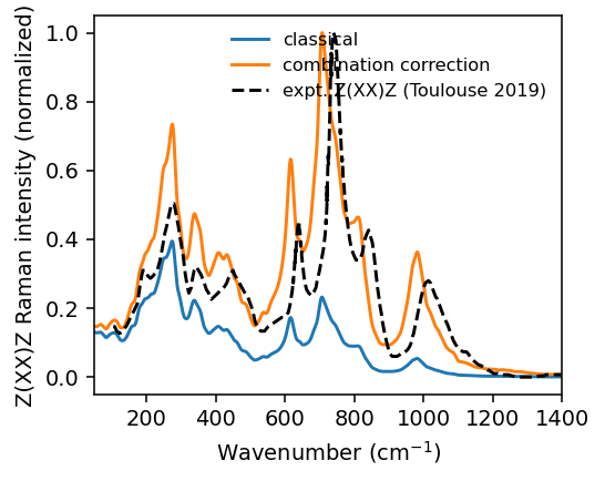
The overall agreement between the TNEP prediction and experiment is good. The broad second-order Raman envelope is reproduced in both shape and frequency range. The higher-frequency features above approximately 600 cm\(^{-1}\) are slightly redshifted relative to experiment, which could be a feature of the exchange-correlation functional used for the underlying density functional theory calculations or the classical treatment. The relative intensities of the low- and high-frequency regions differ slightly from experiment, which could also be caused by a small misalignment of the scattering geometry in the experiment. A detailed discussion is given in Rosander et al. (2025).
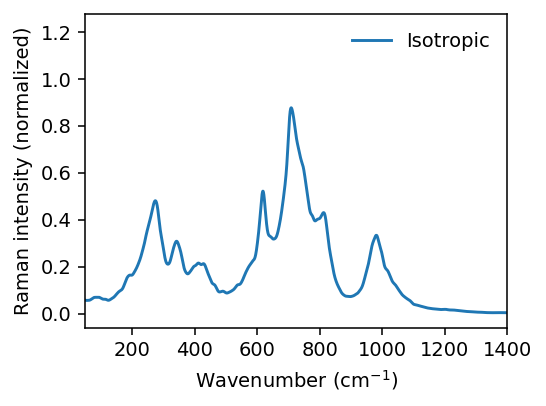
It is also possible to inspect the isotropic Raman spectrum.
[6]:
raman_iso_cb = apply_quantum_correction(
    raman_df, temperature, 'raman_isotropic', order='combination')
[7]:
fig, ax = plt.subplots(figsize=(4, 3), dpi=140)
ax.plot(wn,
        raman_iso_cb['raman_isotropic_qm'] / norm_factor,
        label='Isotropic')
ax.set_xlabel(r'Wavenumber (cm$^{-1}$)')
ax.set_ylabel('Raman intensity (normalized)')
ax.set_xlim(50, 1400)
ax.set_ylim(0, 1)
ax.legend(frameon=False)
fig.tight_layout()
Convergence with run length#
Each pressure above uses a 1 ns run. To see how much this matters, we recompute the spectrum for the 300 K, 0 GPa (cubic) case using only the first 20, 50, 100, 300, or 1000 ps of the same trajectory. We keep the autocorrelation window fixed (20 ps) across all truncations so that what changes between curves is purely the amount of data available to estimate the autocorrelation function, not the frequency resolution. Since window_size is an absolute time in ps rather than a fraction of the
(truncated) trajectory length, it requires no rescaling for each length.
[8]:
lengths_ps = [20, 50, 100, 300, 1000]
window_ps = 20  # fixed autocorrelation window, independent of run length

fig, ax = plt.subplots(figsize=(4, 3.2), dpi=140)
cmap = plt.colormaps['viridis']
for k, length_ps in enumerate(lengths_ps):
    chi_truncated = chi_df[chi_df.time <= length_ps]
    df_k = get_raman_spectrum(chi_truncated, t_sigma=1.0, window_size=window_ps,
                              polarization_in=[1, 0, 0], polarization_out=[1, 0, 0])
    df_k = apply_quantum_correction(df_k, temperature, 'raman_polarized', order='combination')

    wn_k = df_k['wavenumber_invcm']
    mask_k = (wn_k > 600) & (wn_k < 800)
    scale_k = df_k.loc[mask_k, 'raman_polarized_qm'].max()
    ax.plot(wn_k, df_k['raman_polarized_qm'] / scale_k,
            color=cmap(k / (len(lengths_ps) - 1)), label=f'{length_ps} ps')

ax.set_xlabel(r'Wavenumber (cm$^{-1}$)')
ax.set_ylabel('Z(XX)Z Raman intensity (norm.)')
ax.set_xlim(50, 1400)
ax.set_ylim(0, 1.1)
ax.legend(title='Run length', frameon=False, fontsize='small', title_fontsize='small')

fig.tight_layout()
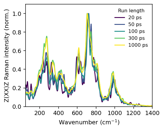
The overall envelope is already recognizable from just 20 ps, but the shorter runs are visibly noisier across the whole second-order band. Longer runs average the autocorrelation function over more statistically independent time origins, giving a cleaner spectrum for the same frequency resolution. The full 1 ns run used elsewhere in this tutorial is comfortably converged by this measure.
Pressure dependence#
We now compute the Raman spectrum at each pressure, track the structural phase transition via the lattice parameters, and compare the second-order (cubic) and first-order (tetragonal) spectra.
[9]:
import re
from glob import glob
from pandas import DataFrame
from calorine.gpumd import read_thermo

dirs = glob(f'{basedir}/300K-*GPa')

results = []
for dname in dirs:
    p_label = float(re.search(r'([\d.]+)GPa', dname).group(1))
    thermo = read_thermo(f'{dname}/thermo.out', normalize=True)
    thermo = thermo[thermo.time > 0.2 * thermo.time.max()]
    abc = sorted([
        (thermo.cell_length_1 / 20).mean(),
        (thermo.cell_length_2 / 20).mean(),
        (thermo.cell_length_3 / 20).mean(),
    ])
    results.append({
        'p_label': p_label,
        'P': thermo.pressure.mean(),
        'V': thermo.volume.mean() / natoms,
        'a': abc[0],
        'b': abc[1],
        'c': abc[2],
    })
averages = DataFrame(results).sort_values('P', ignore_index=True)
averages.head()
[9]:
| p_label | P | V | a | b | c | |
|---|---|---|---|---|---|---|
| 0 | 0.0 | 0.007108 | 14.921185 | 4.208935 | 4.209951 | 4.210406 |
| 1 | 4.0 | 3.977147 | 14.560038 | 4.175038 | 4.175129 | 4.176400 |
| 2 | 8.0 | 7.979239 | 14.237289 | 4.143982 | 4.144430 | 4.144906 |
| 3 | 12.0 | 11.993134 | 13.946974 | 4.115882 | 4.115891 | 4.116454 |
| 4 | 13.0 | 13.042885 | 13.875163 | 4.108634 | 4.108800 | 4.109563 |
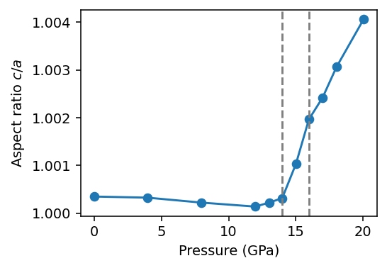
We first inspect the axial ratio as a function of pressure, which reveals the transition pressure. Here, we are satisfied with a rather approximate determination of the transition pressure, which occurs between 14 and 16 GPa. In production this analysis should be done more carefully.
[10]:
fig, ax = plt.subplots(figsize=(4, 2.8), dpi=140)
ax.plot(averages['P'], averages['c'] / averages['a'], 'o-',)
ax.set_xlabel('Pressure (GPa)')
ax.set_ylabel('Aspect ratio $c/a$')
ax.axvline(14, ls='--', color='0.5')
ax.axvline(16, ls='--', color='0.5')
fig.tight_layout()
Now we compute the Raman spectra.
[11]:
spectra = {}
for dname in dirs:
    p_label = float(
        re.search(r'([\d.]+)GPa', dname).group(1))
    chi = read_polarizability(f'{dname}/polarizability.out', normalize=True)
    df = get_raman_spectrum(
        chi, t_sigma=1.0,
        polarization_in=[1, 0, 0], polarization_out=[1, 0, 0])
    df = apply_quantum_correction(
        df, temperature, 'raman_polarized', order='combination')
    spectra[p_label] = df
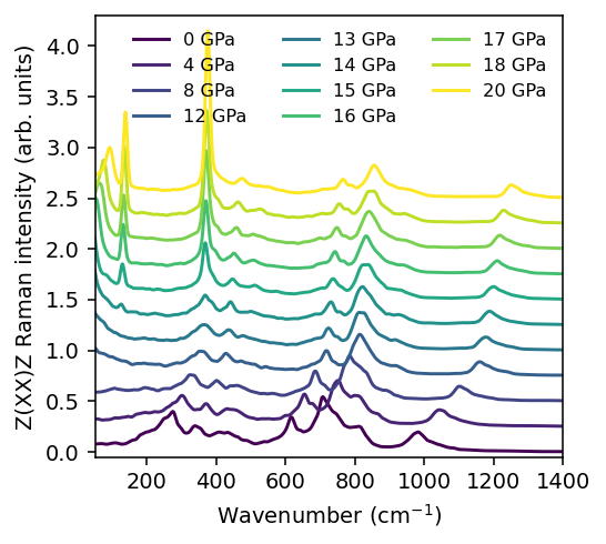
In the result below, we can see that as the pressure passes through the cubic-to-tetragonal phase transition around 14 to 16 GPa, the character of the Raman spectrum changes qualitatively. The broad, relatively weak second-order (two-phonon) scattering of the cubic phase is replaced by intense, narrow first-order peaks in the tetragonal phase. Because all spectra are normalized to a common reference (the maximum of the 0 GPa spectrum), this transition appears as a pronounced jump in absolute intensity in the waterfall plot.
[12]:
p0 = min(spectra)
norm_pres = spectra[p0]['raman_polarized_qm'].max()
offset = 0.25
n_p = len(dirs)
cmap = plt.colormaps['viridis'].resampled(n_p)
wn_all = next(iter(spectra.values()))['wavenumber_invcm']
[13]:
fig, ax = plt.subplots(figsize=(4, 3.6), dpi=140)
for idx, (p_label, df) in enumerate(sorted(spectra.items())):
    y = df['raman_polarized_qm'] / norm_pres + idx * offset
    ax.plot(wn_all, y, color=cmap(idx), label=f'{p_label:.0f} GPa')
ax.set_xlabel(r'Wavenumber (cm$^{-1}$)')
ax.set_ylabel('Z(XX)Z Raman intensity (arb. units)')
ax.set_xlim(50, 1400)
ax.set_ylim(-0.05, 4.3)
ax.legend(frameon=False, fontsize='small', ncol=3)
fig.tight_layout()
Polarized Raman#
In an ordered crystal, Raman spectra can be recorded for specific scattering geometries, revealing the symmetry of individual phonon modes. The geometry is commonly expressed in Porto notation \(A(BC)D\): \(A\) is the propagation direction of the incoming light, \(B\) is the incoming polarization, \(C\) is the outgoing polarization, and \(D\) is the propagation direction of the scattered light.
get_raman_spectrum accepts optional polarization_in and polarization_out unit-vector arguments (corresponding to \(B\) and \(C\)). When both are specified, the function returns a raman_polarized column.
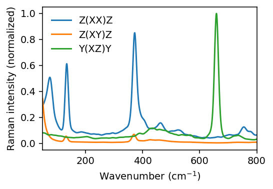
Following Rosander et al. (2025), Fig. 5, we compute three geometries for the tetragonal phase:
Z(XX)Z: both beams along \(z\), both polarized along \(x\) (parallel)
Z(XY)Z: both beams along \(z\), crossed polarizations (perpendicular)
Y(XZ)Y: beams along \(y\), incoming \(x\), outgoing \(z\)
The highest available pressure directory is used as a representative tetragonal-phase simulation (the cubic-to-tetragonal transition occurs at approximately 14 to 16 GPa).
[14]:
folder_tet = f'{basedir}/300K-18GPa'
pol_tet = read_polarizability(f'{folder_tet}/polarizability.out', normalize=True)

geometries = {
    'Z(XX)Z': ([1, 0, 0], [1, 0, 0]),
    'Z(XY)Z': ([1, 0, 0], [0, 1, 0]),
    'Y(XZ)Y': ([1, 0, 0], [0, 0, 1]),
}
pol_spectra = {}
for name, (e_in, e_out) in geometries.items():
    df = get_raman_spectrum(
        pol_tet, t_sigma=1.0,
        polarization_in=e_in,
        polarization_out=e_out,
    )
    df = apply_quantum_correction(df, temperature, 'raman_polarized', order='first')
    pol_spectra[name] = df
[15]:
fig, ax = plt.subplots(figsize=(4, 2.8), dpi=140)
for name, df in pol_spectra.items():
    wn_p = df['wavenumber_invcm']
    y = df['raman_polarized_qm']
    ax.plot(wn_p, y / y.max(), label=name)
ax.set_xlabel(r'Wavenumber (cm$^{-1}$)')
ax.set_ylabel('Raman intensity (normalized)')
ax.set_xlim(50, 800)
ax.legend(frameon=False)
fig.tight_layout()
Discussion#
Second-order vs first-order Raman: At 0 GPa the cubic phase produces a broad second-order (two-phonon) spectrum. Above the cubic-to-tetragonal transition, first-order Raman peaks emerge and are considerably more intense. The lattice-parameter plot shows the onset of the phase transition through the divergence of the \(a\) and \(c\) parameters.
Quantum corrections: Without quantum corrections, classical MD underestimates spectral intensities at high frequencies where \(\hbar\omega \gg k_\mathrm{B}T\). The overtone and combination corrections differ primarily at higher frequencies. The overtone correction falls off more slowly, and the two limiting cases bracket the experimental spectrum, reflecting that the real second-order spectrum is a mixture of both types of processes.
Polarized Raman: Different scattering geometries probe different irreducible representations of the crystal point group. In the tetragonal phase, only modes of specific symmetry contribute to each geometry, making polarized Raman a powerful tool for mode assignment.
A detailed discussion of the computed spectra and their comparison to experiment can be found in Rosander et al., Phys. Rev. B 111, 064107 (2025), and Fransson et al., Chem. Mater. 36, 514 (2024). Experimental Raman spectra for BaZrO\(_3\) at ambient conditions are from Toulouse et al., Phys. Rev. B 100, 134102 (2019).