Using the ASE calculators

This tutorial demonstrates how to use the ASE calculators for neuroevolution potential (NEP) models, which allow one to calculate energies, forces and stresses for an atomic configuration, specified in the form of an Atoms object. This enables one to programmatically calculate properties that would otherwise require writing a large number of GPUMD input files and potentially tedious extraction of the results.

calorine provides two different ASE calculators for NEP calculations, one that uses the GPU implementation and one that uses the CPU implementation of NEP. For smaller calculations the CPU calculator is usually more performant. For very large simulations and for comparison the GPU calculator can be useful as well.

All models and structures required for running this tutorial notebook can be obtained from Zenodo.

import os
import urllib.request
import zipfile

os.makedirs('ase_calculators', exist_ok=True)
base_url = 'https://zenodo.org/records/21198312/files'

# nep-PbTe.txt is shared with other tutorials and lives as a standalone file
fname = 'ase_calculators/nep-PbTe.txt'
if not os.path.exists(fname):
    urllib.request.urlretrieve(f'{base_url}/nep-PbTe.txt', fname)
    print('Downloaded nep-PbTe.txt')
else:
    print('nep-PbTe.txt already present')

# nep-PTAF-dipole.txt + PTAF-monomer.xyz are used exclusively by this tutorial's
# dipole-moment demo, so they are bundled into their own small zip
if not os.path.exists('ase_calculators/nep-PTAF-dipole.txt'):
    urllib.request.urlretrieve(f'{base_url}/ase_calculators_dipole.zip', 'ase_calculators_dipole.zip')
    with zipfile.ZipFile('ase_calculators_dipole.zip') as zf:
        zf.extractall('ase_calculators')
    os.remove('ase_calculators_dipole.zip')
    print('Downloaded and extracted nep-PTAF-dipole.txt, PTAF-monomer.xyz')
else:
    print('nep-PTAF-dipole.txt / PTAF-monomer.xyz already present')

os.chdir('ase_calculators')

Downloaded nep-PbTe.txt
Downloaded and extracted nep-PTAF-dipole.txt, PTAF-monomer.xyz

CPU-based calculator

Basic usage

First we define an atomic structure in the form of an Atoms object. Next we create a calculator instance by specifying the path to a NEP model file in nep.txt format. In this tutorial, we use a NEP4 model for PbTe. Finally, we attach the calculator to the Atoms object.

from ase.io import read
from ase.build import bulk
from calorine.calculators import CPUNEP

structure = bulk('PbTe', crystalstructure='rocksalt', a=6.7)
calc = CPUNEP('nep-PbTe.txt')
structure.calc = calc

Now, we can readily calculate energies, forces and stresses.

print('Energy (eV):', structure.get_potential_energy())
print('Forces (eV/Å):\n', structure.get_forces())
print('Stress (eV/Å^3):\n', structure.get_stress())

Energy (eV): -7.741014073602961
Forces (eV/Å):
 [[ 3.12250226e-16 -2.47895416e-16 -5.04656705e-16]
 [-3.26128013e-16  2.47895416e-16  5.04656705e-16]]
Stress (eV/Å^3):
 [-1.04322062e-02 -1.04322062e-02 -1.04322062e-02  6.32148422e-19
  9.25786486e-18  9.98654588e-18]

Calculate energy-volume curve

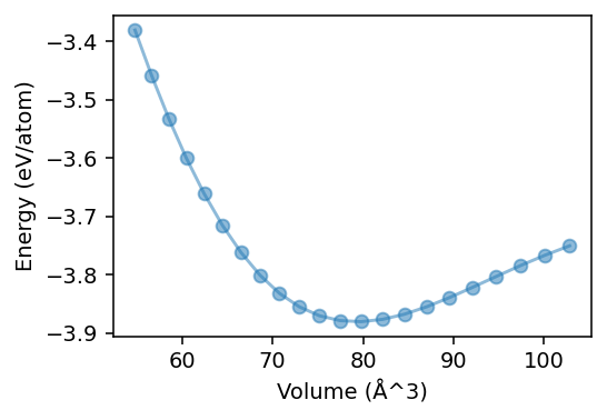
To demonstrate the capabilities of the ASE calculator, we will now calculate an energy-volume curve with the PbTe potential.

%matplotlib inline
import numpy as np
from matplotlib import pyplot as plt

energies = []
volumes = []

structure_copy = structure.copy()
original_cell = structure.cell.copy()

structure_copy.calc = calc

for scale in np.arange(0.9, 1.11, 0.01):
    structure_copy.set_cell(scale * original_cell, scale_atoms=True)
    volumes.append(structure_copy.get_volume())
    energies.append(structure_copy.get_potential_energy() / len(structure_copy))

fig, ax = plt.subplots(figsize=(4, 2.8), dpi=140)

ax.plot(volumes, energies, '-o', alpha=0.5)
ax.set_xlabel('Volume (Å^3)')
ax.set_ylabel('Energy (eV/atom)')

fig.tight_layout()

Structure relaxation

calorine.tools.relax_structure relaxes a structure’s atomic positions and, optionally, its cell using the attached calculator. It is a thin wrapper around the optimizers in the ase package. To demonstrate the effect, we build a slightly strained structure and print the pressure before and after relaxation.

import numpy as np
from ase.units import GPa
from calorine.tools import relax_structure

structure = bulk('PbTe', crystalstructure='rocksalt', a=6.6)
calc = CPUNEP('nep-PbTe.txt')
structure.calc = calc

pressure = -np.sum(structure.get_stress()[:3]) / 3 / GPa
print(f'Pressure before: {pressure:.2f} GPa')

relax_structure(structure)
pressure = -np.sum(structure.get_stress()[:3]) / 3 / GPa
print(f'Pressure after:  {pressure:.2f} GPa')

Pressure before: 3.36 GPa
Pressure after:  0.00 GPa

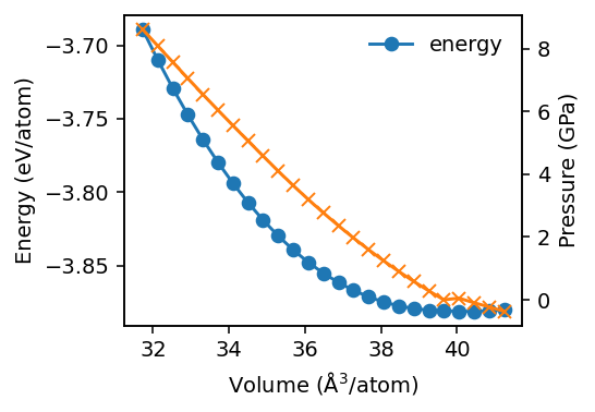
The energy-volume curve above scanned a rigid, uniform volume strain without relaxing the atomic positions or cell shape at each point. For a more accurate curve, relax_structure can be called at fixed volume (constant_volume=True, which allows the atomic positions and the cell shape to relax while keeping the volume fixed) at each point of the scan.

%%time

from pandas import DataFrame

data = []
for volsc in np.arange(0.8, 1.05, 0.01):
    s = structure.copy()
    # the cubic root converts from volume strain to linear strain
    s.cell *= volsc ** (1 / 3)
    s.calc = calc
    relax_structure(s, constant_volume=True)
    data.append(dict(volume=s.get_volume() / len(structure),
                     energy=s.get_potential_energy() / len(structure),
                     pressure=-np.sum(s.get_stress()[:3]) / 3 / GPa))
df = DataFrame.from_dict(data)

CPU times: user 5.07 s, sys: 6.13 ms, total: 5.07 s
Wall time: 1.69 s

fig, ax = plt.subplots(figsize=(4, 2.8), dpi=140)

ax.plot(df.volume, df.energy, 'o-', label='energy')
ax2 = ax.twinx()
ax2.plot(df.volume, df.pressure, 'x-', color='C1', label='pressure')

ax.set_xlabel('Volume (Å$^3$/atom)')
ax.set_ylabel('Energy (eV/atom)')
ax2.set_ylabel('Pressure (GPa)')
ax.legend(frameon=False)

fig.tight_layout()

Relaxation with a fixed cell

In some scenarios, it is helpful to keep the cell constant but still relax the atomic configuration. This can be done by setting the constant_cell keyword argument. We save the cell and atomic positions before relaxing, then confirm that the atoms moved but the cell did not change.

structure = bulk('PbTe', crystalstructure='rocksalt', a=6.6)
structure.cell *= 1.1 ** (1 / 3)  # we strain the cell like above
structure.calc = CPUNEP('nep-PbTe.txt')

positions_pre_relax = structure.get_positions()
cell_pre_relax = structure.get_cell()

relax_structure(structure, constant_cell=True)

assert not np.allclose(positions_pre_relax, structure.get_positions())
assert np.allclose(cell_pre_relax, structure.get_cell())
print('Atoms moved; cell unchanged, as expected.')

Atoms moved; cell unchanged, as expected.

Calculate dipole moments

The calculator also supports the calculation of dipole moments. You must have a tensorial NEP (TNEP) trained to predict dipoles; otherwise the output will be nonsensical. Refer to this TNEP training tutorial for information on how to train a TNEP model for rank-1 tensors such as the dipole or the polarization.

dipole_model = 'nep-PTAF-dipole.txt'
structure = read('PTAF-monomer.xyz')
calc = CPUNEP(dipole_model)
structure.calc = calc

dipole = structure.get_dipole_moment()
dft_dipole = structure.info['dipole_moment']

print('DFT dipole moment:'.ljust(30) +  f'{dft_dipole} a.u.')
print('NEP predicted dipole moment:'.ljust(30) + f'{dipole} a.u.')

DFT dipole moment:            [4.85503 0.07166 0.16004] a.u.
NEP predicted dipole moment:  [4.78034782 0.03274603 0.04843106] a.u.

GPU-based calculator

The basic usage of the GPUNEP calculator class is completely analogous to the CPUNEP calculator. We create an atomic structure and attach the calculator object.

from calorine.calculators import GPUNEP

structure = bulk('PbTe', crystalstructure='rocksalt', a=6.7)
calc = GPUNEP('nep-PbTe.txt')
structure.calc = calc

Afterwards we can readily obtain energies, forces, and stresses.

print('Energy (eV):', structure.get_potential_energy())
print('Forces (eV/Å):\n', structure.get_forces())
print('Stress (eV/Å^3):\n', structure.get_stress())

Energy (eV): -7.7410137653
Forces (eV/Å):
 [[ 1.29556555e-07  2.14915124e-07  1.63774920e-07]
 [-1.29556555e-07 -2.14915124e-07 -1.63774920e-07]]
Stress (eV/Å^3):
 [-1.04321760e-02 -1.04321839e-02 -1.04321777e-02  7.17762087e-10
  4.00239732e-10 -2.93254915e-09]

By default, GPUNEP runs the gpumd executable found on your PATH. If you need to point it at a different binary or wrapper script (e.g., a specific build, or a script that loads environment modules before launching GPUMD on a cluster), you can set the CALORINE_GPUMD_COMMAND environment variable. GPUNEP falls back to the literal 'gpumd' command when it is unset. You can also pass an explicit command= argument to the GPUNEP constructor, which takes precedence over the environment variable.

Precision and speed

GPUNEP uses the implementation in GPUMD, which computes in single precision (float32) for performance; CPUNEP on the other hand uses the double-precision (float64). For most applications (relaxation, MD, elastic/phonon properties at typical tolerances) the resulting differences in energies and forces are negligible, but it is worth being aware of when you need very small forces to converge tightly (e.g., strict relaxation tolerances or finite-difference derivatives). If in doubt compare CPUNEP and GPUNEP on the same structure.

The trade-off in speed goes the other way: CPUNEP is faster for small structures, since GPUNEP pays a fixed overhead for launching GPUMD as a subprocess and transferring data, while GPUNEP overtakes it as the system size grows because the NEP evaluation parallelizes efficiently across atoms on the GPU. The cell below benchmarks both across a range of supercell sizes.

import time

sizes = [1, 2, 3, 4, 6, 8, 10, 16, 24, 36, 48]
natoms_list, cpu_times, gpu_times = [], [], []

for size in sizes:
    bench_structure = bulk('PbTe', crystalstructure='rocksalt', a=6.7).repeat(size)
    natoms_list.append(len(bench_structure))

    bench_structure.calc = CPUNEP('nep-PbTe.txt')
    t0 = time.perf_counter()
    bench_structure.get_potential_energy()
    cpu_times.append(time.perf_counter() - t0)

    bench_structure.calc = GPUNEP('nep-PbTe.txt')
    t0 = time.perf_counter()
    bench_structure.get_potential_energy()
    gpu_times.append(time.perf_counter() - t0)

    print(f'{natoms_list[-1]:6} atoms: CPU {cpu_times[-1]:.3f} s, GPU {gpu_times[-1]:.3f} s')

     2 atoms: CPU 0.001 s, GPU 0.280 s
    16 atoms: CPU 0.002 s, GPU 0.251 s
    54 atoms: CPU 0.003 s, GPU 0.251 s
   128 atoms: CPU 0.007 s, GPU 0.256 s
   432 atoms: CPU 0.019 s, GPU 0.271 s
  1024 atoms: CPU 0.043 s, GPU 0.259 s
  2000 atoms: CPU 0.080 s, GPU 0.251 s
  8192 atoms: CPU 0.347 s, GPU 0.298 s
 27648 atoms: CPU 1.137 s, GPU 0.463 s
 93312 atoms: CPU 3.665 s, GPU 0.924 s
221184 atoms: CPU 11.174 s, GPU 1.761 s
   128 atoms: CPU 0.007 s, GPU 0.249 s
   432 atoms: CPU 0.019 s, GPU 0.247 s
  1024 atoms: CPU 0.046 s, GPU 0.251 s
  2000 atoms: CPU 0.082 s, GPU 0.243 s
  8192 atoms: CPU 0.372 s, GPU 0.303 s
 27648 atoms: CPU 1.174 s, GPU 0.426 s
 93312 atoms: CPU 3.797 s, GPU 0.959 s
221184 atoms: CPU 9.556 s, GPU 1.780 s

fig, ax = plt.subplots(figsize=(4, 2.8), dpi=140)

ax.plot(natoms_list, cpu_times, 'o-', label='CPUNEP')
ax.plot(natoms_list, gpu_times, 's-', label='GPUNEP')
ax.set_xlabel('Number of atoms')
ax.set_ylabel('Wall time (s)')
ax.set_xscale('log')
ax.set_yscale('log')
ax.legend(frameon=False)

fig.tight_layout()

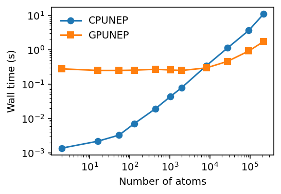
In this benchmark CPUNEP outperforms GPUNEP up to roughly 10,000 atoms. This is not a measurement of raw GPUMD performance: GPUNEP pays a fixed overhead for launching GPUMD as a subprocess and writing/reading its input and output files on every single call. Its cost therefore stays roughly flat up to about 20,000 atoms, while the cost of CPUNEP scales up already from a few tens of atoms. If you run an actual MD simulation directly through GPUMD (as in the section below), rather than calling GPUNEP once per structure, you avoid this per-call overhead entirely and GPUMD is much faster.

Temporary and specified directories

Under the hood, the GPUNEP calculator creates a directory and writes the input files necessary to run GPUMD. By default, this is done in temporary directories that are automatically removed once the calculation has finished. It is also possible to run in a user-specified directory that will be kept after the calculations finish. This is especially useful when running molecular dynamics simulations (see below).

calc.set_directory('my_directory')
structure.get_potential_energy()

np.float64(-7.7410137653)

After this is run, there should be a new directory, my_directory, in which input and output files from GPUMD are available. This can be useful for debugging.

Running custom molecular dynamics simulations

To take advantage of the Python workflow as well as raw speed of the GPU accelerated NEP implementation, the GPUNEP calculator contains a convenience function for running customized molecular dynamics simulations. This should typically be done in a specified directory. The parameters of the run.in file are specified as a list of tuples with two elements, the first being the keyword name and the second any arguments to that keyword.

%%time

import shutil
from ase.build import make_supercell

# Create a cubic supercell from the FCC-shaped primitive cell
P = [[-1, 1, 1], [1, -1, 1], [1, 1, -1]]
supercell = make_supercell(structure, P).repeat(12)

# Start from a clean directory
shutil.rmtree('my_md_simulation', ignore_errors=True)

# Launch MD
calc.set_directory('my_md_simulation')
supercell.calc = calc
parameters = [('velocity', 300),
              ('dump_thermo', 100),
              ('dump_position', 100),
              ('ensemble', ('nvt_lan', 300, 300, 100)),
              ('run', 20000)]
calc.run_custom_md(parameters)

CPU times: user 63 ms, sys: 2.23 ms, total: 65.2 ms
Wall time: 18.1 s

Once this is run, the results are available in the folder my_md_simulation.

Analyzing the trajectory

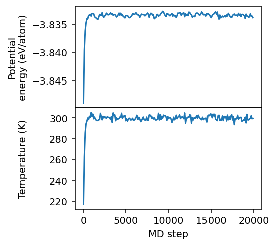
A minimal follow-up to any MD run is to check that the simulation is well-behaved by loading the thermodynamic quantities written to thermo.out and plotting them against simulation time. A dedicated tutorial on analyzing MD trajectories in more depth does not exist yet; this is just a quick sanity check.

from calorine.gpumd.io import read_thermo

thermo = read_thermo('my_md_simulation/thermo.out', natoms=len(supercell))
steps = 100 * np.arange(len(thermo))  # dump_thermo every 100 steps (see cell above)

fig, axes = plt.subplots(figsize=(4, 3.6), nrows=2, sharex=True, dpi=140)

axes[0].plot(steps, thermo['potential_energy'])
axes[0].set_ylabel('Potential\nenergy (eV/atom)')

axes[1].plot(steps, thermo['temperature'])
axes[1].set_ylabel('Temperature (K)')
axes[1].set_xlabel('MD step')

fig.tight_layout()
fig.subplots_adjust(hspace=0)
fig.align_labels()

Using a foundation model

All of the above works identically with any NEP model file, including large general-purpose “foundation” models trained across much of the periodic table, such as NEP89 (also available from the same Zenodo record as nep89.txt). These are convenient when no system-specific model exists yet, at some cost in accuracy relative to a model trained specifically for your system of interest.