Inelastic neutron scattering spectra

This tutorial implements a simplified and minimal version of the workflow presented in the article by Lindgren et al. (2025) for simulating inelastic neutron scattering spectra (INS) from first principles. Specifically, this notebook demonstrates how to run molecular dynamics (MD) simulations using a NEP model for crystalline benzene, compute the INS spectrum from the dynamic structure factor, and correct for the instrument resolution and kinematic constraint in order to compare to experimentally measured spectra. We compare to the INS spectrum measured at the TOSCA spectrometer at the ISIS Neutron and Muon Source in the UK, published in the preprint by Lindgren et al.

In addition to the requirements for calorine, this tutorial requires installation of the following packages:

• dynasor Link: pip install dynasor

• euphonic Link: pip install euphonic

• resINS Link: pip install resins

The data required for running this tutorial notebook can be obtained from Zenodo.

import os
import zipfile
import urllib.request

url = 'https://zenodo.org/records/21198312/files/inelastic_neutron_scattering.zip'
if not os.path.exists('inelastic_neutron_scattering'):
    urllib.request.urlretrieve(url, 'inelastic_neutron_scattering.zip')
    with zipfile.ZipFile('inelastic_neutron_scattering.zip') as zf:
        zf.extractall('.')
    os.remove('inelastic_neutron_scattering.zip')
    print('Downloaded and extracted inelastic_neutron_scattering/')
else:
    print('inelastic_neutron_scattering/ already present')
os.chdir('inelastic_neutron_scattering')

Downloaded and extracted inelastic_neutron_scattering/

Preparations

We begin by loading a primitive benzene structure in the I phase and the NEP model nep-benzene.txt, both originally from the Zenodo record from Lindgren et al. (2025). We then use the NEP model to relax the primitive structure.

import numpy as np
from ase.io import read, write
from calorine.calculators import CPUNEP
from calorine.tools import relax_structure

primitive = read('benzene-I.xyz')
potential = './nep-benzene.txt'
calculator = CPUNEP(potential)
primitive.calc = calculator

from ase.constraints import FixSymmetry
from calorine.tools import get_spacegroup

# Relax the structure
epot = primitive.get_potential_energy() / len(primitive)
spg = get_spacegroup(primitive)
print(f'Before relaxation : energy = {epot:.3f} eV/atom; spacegroup  = {spg}')

# Apply constraint so that the symmetry is preserved during relaxation
primitive.set_constraint(FixSymmetry(primitive))
relax_structure(primitive, minimizer='bfgs-scipy', fmax=1e-3)

epot = primitive.get_potential_energy() / len(primitive)
print(f'After relaxation  : energy = {epot:.3f} eV/atom; spacegroup  = {spg}')

# Remove constraint since it is not needed anymore
primitive.set_constraint()

# Make spurious components of cell metric that
# are very close to zero, strictly zero.
primitive.cell[np.abs(primitive.cell) < 1e-6] = 0

Before relaxation : energy = -5.390 eV/atom; spacegroup  = Pbca (61)
After relaxation  : energy = -5.726 eV/atom; spacegroup  = Pbca (61)

Next, we will set up the supercell for molecular dynamics. We will use a relatively small system size for the purpose of this tutorial. The supercell is created such that the cell vectors are approximately of equal length.

# Set up the supercell for molecular dynamics
repeats = (6, 4, 6)
supercell = primitive.repeat(repeats)
print('Number of atoms in supercell:', len(supercell))
print('Cell vector lengths in supercell (Å):', supercell.cell.lengths())

Number of atoms in supercell: 6912
Cell vector lengths in supercell (Å): [43.2907884  37.93322221 42.20063446]

Molecular dynamics

We are now ready to run the molecular dynamics simulation. As for any GPUMD simulation, this requires a structure file (model.xyz) and a set of run instructions (run.in). The simulation protocol is divided into two parts. First, we perform an equilibration run to get the correct simulation cell at the target conditions of 127 K and a pressure of 0 GPa. From the last part of the equilibration trajectory we then extract the average simulation cell, and use it to set up a production run, where the atomic positions are written with a high frequency of every 4 fs.

This high frequency is required for the next step of the workflow, where we compute the dynamic structure factor. It is paramount to write sufficiently often, such that all vibrational modes are sampled at least twice per period according to the Nyquist sampling theorem. In our system, the fastest mode is the C-H stretching mode, which has an energy of ~3200 cm\(^{-1}\) or 400 meV, equivalent to a period time of 10.5 fs. Writing the trajectory file every 4 fs is thus sufficient to respect the Nyquist condition.

Both runs are set up as regular GPUMD jobs, with input files (run.in, and, for equilibration, model.xyz) provided in the equilibration/ and production/ subdirectories. If you want to reproduce or extend the results, you can run these yourself, e.g.

cd equilibration && gpumd

(and similarly for production, once its model.xyz has been generated below). On a GH200 GPU the runs take about 6 and 4 minutes, respectively, for equilibration and production.

To avoid accidentally overwriting the precomputed data used in the analysis below, reference results are stored in equilibration/example-output/ and production/example-output/, rather than directly in equilibration//production/. The analysis below reads from example-output/ by default. Point it at the plain equilibration//production/ directories instead if you ran your own job.

write('equilibration/model.xyz', supercell)
print(open('equilibration/run.in').read())

potential ../nep-benzene.txt
time_step 0.5
velocity 200

ensemble nvt_lan 127 127 100
dump_thermo   200
run         20000

ensemble npt_scr 127 127 100 0 0 0 40 40 40 200
dump_thermo   200
dump_exyz   20000
run        100000

We quickly check the thermo.out file in equilibration/example-output/ to ensure that the structure is properly equilibrated before we move on to production.

import numpy as np
from calorine.gpumd.io import read_thermo
from matplotlib import pyplot as plt

# Use our precomputed example output by default. If you ran your own equilibration job
# (see equilibration/run.in), point this at 'equilibration' instead.
equilibration_dir = 'equilibration/example-output'

natoms = len(supercell)
thermo = read_thermo(f'{equilibration_dir}/thermo.out', natoms=natoms)
# in fs, thermo is written every 100 steps = 10 fs
time = np.linspace(0, len(thermo)*10, len(thermo))

fig, axes = plt.subplots(figsize=(4, 5.6), nrows=4, sharex=True, dpi=140)

# Potential energy
ax = axes[0]
ax.plot(time, thermo['potential_energy'])
ax.set_ylabel('Pot. energy\n (eV/atom)')

# Temperature
ax = axes[1]
ax.plot(time, thermo['temperature'])
ax.set_ylabel('Temperature (K)')

# Cell volume
ax = axes[2]
a = np.array(thermo['cell_xx'])
b = np.array(thermo['cell_yy'])
c = np.array(thermo['cell_zz'])
V = a * b * c

ax.plot(time, a / repeats[0])
ax.plot(time, b / repeats[1])
ax.plot(time, c / repeats[2])
ax.set_ylabel('Cell (Å)')

# Pressure
ax = axes[3]
P = -1 / 3 * (thermo['stress_xx'] + thermo['stress_yy'] + thermo['stress_zz'])
ax.plot(time, P)
ax.set_ylabel('Pressure (GPa)')
ax.set_xlabel('Time (fs)')

fig.tight_layout()
fig.subplots_adjust(wspace=0, hspace=0)
fig.align_labels()

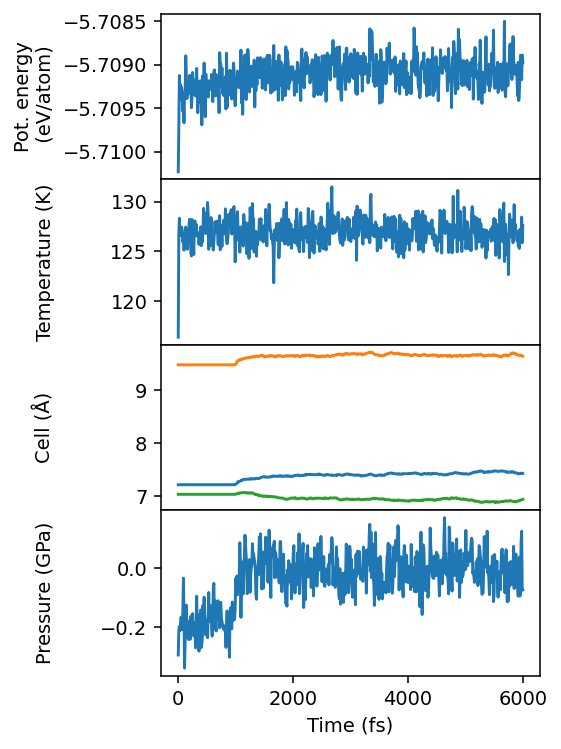
The results show that the cell lengths, temperature, and pressure have all converged to stable averages.

We now build the starting configuration for the production run: the last frame of the equilibration trajectory, with its cell replaced by the average of the last 100 observations from thermo.out (to average out thermal fluctuations in the cell metric).

df = read_thermo(f'{equilibration_dir}/thermo.out', natoms=natoms)
cell_xx = df.cell_xx.iloc[-100:].mean()
cell_yy = df.cell_yy.iloc[-100:].mean()
cell_zz = df.cell_zz.iloc[-100:].mean()
cell = [cell_xx, cell_yy, cell_zz]

equilibrated = read(f'{equilibration_dir}/dump.xyz')
equilibrated.set_cell(cell, scale_atoms=True)
os.makedirs('production', exist_ok=True)
write('production/model.xyz', equilibrated)

Now, we can run the production run, in the microcanonical (NVE) ensemble. The NVE ensemble is suitable for production as there is no interference on the dynamics of the atoms from a thermostat or barostat. The system is first equilibrated quickly in the NVT ensemble for a short time, then transitioned to the NVE ensemble where positions are written every 4 fs (i.e., dump_exyz 8 times time_step 0.5).

As above, this is a regular GPUMD job (production/run.in, with model.xyz generated above); run it yourself with cd production && gpumd if desired. The analysis below uses the reference results in production/example-output/.

print(open('production/run.in').read())

potential ../nep-benzene.txt
time_step 0.5
velocity 200

ensemble nvt_lan 127 127 100
dump_thermo    200
run          20000

ensemble nve
dump_thermo    200
dump_exyz        8
run          40000

Compute the dynamic structure factor

We now compute the dynamic structure factor \(S(q, \omega)\) using dynasor. The dynamic structure factor is directly proportional to the intensity measured in a scattering experiment, and can be compared to experimental measurements by weighting with appropriate scattering lengths or structure factors.

The computation itself involves generating 1000 randomly selected \(q\)-points up to a maximum value of \(q_\mathrm{max}=12\) rad/Å (a range suitable for the TOSCA spectrometer at the ISIS Neutron and Muon Source, which we compare to below) and evaluating compute_dynamic_structure_factors over the full production trajectory. This takes about 32 minutes on a workstation with a i7-9700 CPU, so it is not run inline in this notebook. Instead, it is computed by the companion script run-dynasor-analysis.py, which reads production/example-output/model.xyz and production/example-output/dump.xyz and writes the result to sample.npz; that file is already included in the data downloaded above, but if you ran your own production job you can regenerate it by running

python run-dynasor-analysis.py

from a terminal in this notebook’s working directory. This script is also a good starting point for setting up your own custom analysis scripts.

sample.npz can be loaded directly as a dynasor Sample object via read_sample_from_npz.

from dynasor import read_sample_from_npz
from dynasor.sample import DynamicSample

sample = read_sample_from_npz('sample.npz')

Finally, we compute and apply neutron scattering lengths to the dynamic structure factor in our Sample object, and perform a spherical average over the q-points. The averaging is performed by applying a Gaussian smearing, here with a width of 0.01 rad/Å, to the \(q\)-points.

from dynasor.post_processing import (
    NeutronScatteringLengths,
    get_weighted_sample,
    get_spherically_averaged_sample_smearing,
)


def weight_and_average_sample(
    sample, q_max: float, q_width: float, n_points: int,
):
    """
    Weights a dynasor sample with neutron scattering lengths, and then
    performs a spherical averaging in q by applying a Gaussian smearing.
    Returns a weighted Dynasor Sample.
    """
    species = sample.atom_types
    weights = NeutronScatteringLengths(species)
    weighted = get_weighted_sample(sample, weights)

    q_norms = np.linspace(0, q_max, n_points)
    smeared = get_spherically_averaged_sample_smearing(
        weighted, q_norms, q_width=q_width  # in rad/Å
    )

    # Finally, compute the total dynamic structure factor Sqw
    # by summing the weighted coherent Sqw_coh and the incoherent Sqw_incoh.
    Sqw = smeared.Sqw_coh + smeared.Sqw_incoh
    smeared.Sqw = Sqw

    return smeared


weighted_and_averaged = weight_and_average_sample(
    sample, q_max=12, q_width=0.01, n_points=400)

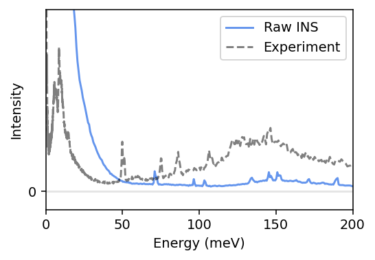
We can now plot the ‘raw’ simulated inelastic neutron scattering spectrum by averaging the dynamic structure factor \(S(q, \omega)\) over \(q\). We skip plotting the elastic line \(S(q, \omega=0)\) as the intensity is very large compared to the rest of the spectrum. We also plot experimental data from Lindgren et al. for comparison.

from dynasor.units import radians_per_fs_to_meV
from scipy.optimize import minimize

# Load experimental data
cm_to_mev = 123.98419 / 1e3  # 1/cm -> meV
exp = np.loadtxt('data.benzene-tosca-Skoro-Rudic-2019-original-127K',
                 skiprows=1, delimiter=',')
experiment_spectrum = exp[:, -2]
experiment_energy = exp[:,0] * cm_to_mev


def scale_spectrum(simulation, simulation_energy, experiment,
                   experiment_energy, min_energy, max_energy):
    #indices = np.argsort(np.abs(simulation_energy - selected_energy))
    indices = np.argwhere((simulation_energy < max_energy) &
                          (simulation_energy > min_energy))

    interpolated_experiment = np.interp(simulation_energy, experiment_energy, experiment)
    min_obj = minimize(fun=lambda x, spectra, ref: np.mean((x[0]*spectra - ref)**2),
                   x0=[1],
                   args=(simulation[indices], interpolated_experiment[indices]))
    return simulation * min_obj.x[0]

ins_raw = np.nansum(weighted_and_averaged.Sqw, axis=0)
energy = weighted_and_averaged.omega * radians_per_fs_to_meV

ins_raw = scale_spectrum(ins_raw, energy, experiment_spectrum, experiment_energy, 25, 200)

fig, ax = plt.subplots(figsize=(4, 2.8), dpi=140)

ax.plot(energy[1:], ins_raw[1:], c='cornflowerblue', label='Raw INS')
ax.plot(experiment_energy, experiment_spectrum,
        'k--', alpha=0.5, label='Experiment')
ax.axhline(0, c='k', alpha=0.1)
ax.set_xlabel('Energy (meV)')
ax.set_ylabel('Intensity')
ax.set_yticks([0])
ax.legend(loc='upper right')
ax.set_xlim([0, 200])
ax.set_ylim([-1, 10])

fig.tight_layout()

Apply experimental kinematic constraint and resolution function

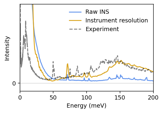
The simulated INS spectrum above does not agree that well with experiments. In order to obtain a good agreement, we need to consider the actual instrument at which the experiment was performed, as well as compensate for the classical statistics from molecular dynamics simulations.

As stated previously, in this case we compare to experimental data measured at the TOSCA spectrometer at the ISIS Neutron and Muon Source in the UK. We use the euphonic and resINS packages to apply the instrument resolution and kinematic constraint.

import warnings
from euphonic import ureg
from euphonic.spectra import Spectrum1D, Spectrum2D, apply_kinematic_constraints
from resins.instrument import Instrument
from scipy.signal import fftconvolve

def resolution_function(sample: DynamicSample, instrument_string: str):
    q_norms = sample.q_norms
    e = radians_per_fs_to_meV * sample.omega
    Sqw = sample.Sqw

    q_norms_spacing = np.mean(np.diff(q_norms))
    q_norm_bin_edges = np.concatenate(
        [[q_norms[0] - q_norms_spacing/2], q_norms + q_norms_spacing/2])
    bin_widths = np.diff(q_norm_bin_edges)

    e_spacing = np.mean(np.diff(e))
    e_bin_edges = np.concatenate([[e[0] - e_spacing/2], e + e_spacing/2])

    spectrum = Spectrum2D(x_data=q_norm_bin_edges*ureg('1/angstrom'),
                          y_data=(e_bin_edges * ureg('meV')),
                          z_data=Sqw*ureg('dimensionless'))
    spectrum.y_data_unit = 'meV'

    instrument = Instrument.from_default(instrument_string)

    if instrument_string == 'TOSCA':
        res_function = 'AbIns'
        E_FINAL = 3.97 * ureg('meV')
        E_INITIAL = None
        # Technically the two detector banks of TOSCA corresponds to
        # the angles 35 and 135 degrees. However, we use two slightly
        # larger angle ranges in order to obtain better statistics.
        angle_range_1 = (30, 40)
        angle_range_2 = (130, 140)
    res_model_mev = instrument.get_resolution_function(
        'AbINS', e_initial=E_INITIAL, e_final=E_FINAL).polynomial


    broadened = spectrum.broaden(
        x_width=1e-1*ureg('1/angstrom'),
        y_width=lambda e: res_model_mev(e.to('meV').magnitude) * ureg('meV'),
        width_convention='std',
        method='convolve')
    constrained_1 = apply_kinematic_constraints(
        broadened, e_f=E_FINAL, angle_range=angle_range_1)
    constrained_2 = apply_kinematic_constraints(
        broadened, e_f=E_FINAL, angle_range=angle_range_2)

    def convolve(constrained):
        # convolve with a Gaussian to simulate less sharp angles
        # Multiply wiht a N(0, 1) and transform to energy units
        def gaussian(slice, x):
            # Convolute a slice of Sqw with a Gaussian
            smear = 0.5      # 1/Å or meV
            # center the convolution gaussian on the maximum intensity
            mu = x[np.argmax(slice)]
            angular_smearing = np.exp( - (x - mu)**2 / (2*smear**2) )
            return fftconvolve(slice, angular_smearing, mode='same')

        non_nan = np.nan_to_num(constrained.z_data.magnitude, nan=0.0)
        q = constrained.x_data.magnitude
        w = constrained.y_data.magnitude
        conv = np.apply_along_axis(gaussian, 0, non_nan, q)  # Apply convolution along q
        return conv

    convolved_intensity_1 = convolve(constrained_1)
    convolved_intensity_2 = convolve(constrained_2)

    kinematic_Sqw = np.nan_to_num(
        constrained_1.z_data, nan=0.0) + np.nan_to_num(constrained_2.z_data, nan=0.0)
    #kinematic_Sqw = convolved_intensity_1 + convolved_intensity_2
    kinematic_Sqw[kinematic_Sqw == 0.0] = np.nan
    #kinematic_Sqw = broadened.z_data

    # Sum the results from the two banks
    constrained = Spectrum2D(
        x_data=broadened.x_data,
        y_data=broadened.y_data,
        z_data=kinematic_Sqw*ureg('dimensionless')
    )

    Sqw = constrained

    # Set x and y points to be bin centers instead of edges
    Sqw.x_data = q_norms * ureg('1/angstrom')
    Sqw.y_data = e * ureg('meV')

    # Compute 1D sample
    # Numpy will throw a warning regarding nanmean here, which we suppress.
    with warnings.catch_warnings():
        warnings.simplefilter('ignore', category=RuntimeWarning)
        Sw = Spectrum1D(x_data=e * ureg('meV'), y_data=np.nanmean(Sqw.z_data, axis=0))
    return Sw.y_data.magnitude, Sw.x_data.magnitude


ins_instrument, _ = resolution_function(weighted_and_averaged, 'TOSCA')

ins_instrument = scale_spectrum(
    ins_instrument, energy, experiment_spectrum,
    experiment_energy, 25, 200)

fig, ax = plt.subplots(figsize=(4, 2.8), dpi=140)

ax.plot(energy[1:], ins_raw[1:],
        c='cornflowerblue', label='Raw INS')
ax.plot(energy[1:], ins_instrument[1:],
        c='goldenrod', label='Instrument resolution')
ax.plot(experiment_energy, experiment_spectrum, 'k--',
        alpha=0.5, label='Experiment')

ax.axhline(0, c='k', alpha=0.1)
ax.set_xlabel('Energy (meV)')
ax.set_ylabel('Intensity')
ax.set_yticks([0])
ax.set_xlim([0, 200])
ax.set_ylim([-1, 10])
ax.legend(frameon=False)

fig.tight_layout()

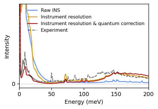
Finally, we compensate for the classical statistics from molecular dynamics simulations by applying a first-order correction factor from perturbation theory. With the correction, we arrive at a semiquantitative prediction of the INS spectrum for crystalline benzene. The remaining red-shift of about 25 meV is attributed to the DFT functional used to train the NEP model. For more information about the correction as well as an extended discussion on the red-shift, please refer to the paper mentioned in the introduction of this tutorial.

from ase.units import kB

def first_order_quantum_correction(energy_in_meV, T):
    """
    Calculates a quantum correction to the classical MD statistics.
    The correction is equal to the Bose-einstein distribution.
    Returns a correction in meV.

    The first order correction is
        corr(e) = beta * e * [n(e) + 1]
                = beta * e / (1 - exp( -beta*e ) )
        n(e) = 1 / ( exp(beta*e) - 1 )
    """

    epsilon = 1e-12  # To avoid division by 1
    e_eV = energy_in_meV * 1e-3  # to eV
    beta = 1 / (kB * T)  # 1/eV
    expon = np.exp( - (e_eV + epsilon) * beta )
    denominator = 1 - expon

    correction = beta * e_eV / denominator
    return correction


def apply_first_order_quantum_correction(simulated, simulated_energy, temperature):
    correction = first_order_quantum_correction(simulated_energy, temperature)
    return simulated*correction

temperature = 127
ins_instrument_and_quantum = apply_first_order_quantum_correction(
    ins_instrument, energy, temperature)

ins_instrument_and_quantum = scale_spectrum(
    ins_instrument_and_quantum, energy,
    experiment_spectrum, experiment_energy, 25, 200)

fig, ax = plt.subplots(figsize=(4, 2.8), dpi=140)

ax.plot(energy[1:], ins_raw[1:], c='cornflowerblue', label='Raw INS')
ax.plot(energy[1:], ins_instrument[1:],
        c='goldenrod', label='Instrument resolution')
ax.plot(energy[1:], ins_instrument_and_quantum[1:],
        c='firebrick', label='Instrument resolution & quantum correction')
ax.plot(experiment_energy, experiment_spectrum, 'k--',
        alpha=0.5, label='Experiment')

ax.axhline(0, c='k', alpha=0.1)
ax.set_xlabel('Energy (meV)')
ax.set_ylabel('Intensity')
ax.set_yticks([0])
ax.set_xlim([0, 200])
ax.set_ylim([-1, 20])
ax.legend(frameon=False, fontsize='small')

fig.tight_layout()

Below is a production-grade simulation of the INS spectrum for benzene from the article by Lindgren et al. (2025). The structure was equilibrated using path-integral molecular dynamics (PIMD) for 500 ps, with production for 1 ns in the NVE ensemble. The system consisted of a 11x9x12 supercell for a total of 57024 atoms.