TNEP model for the susceptibility

Introduction

Raman spectroscopy probes vibrational modes that modulate the electric susceptibility \(\boldsymbol{\chi}\) of a material. The Raman intensity is proportional to the power spectral density of the time derivative of \(\boldsymbol{\chi}(t)\), evaluated along a molecular dynamics trajectory. \(\boldsymbol{\chi}\) is a rank-2 tensor; the TNEP framework captures this with model_type 2, which trains a model that predicts the full \(3 \times 3\) susceptibility tensor for each configuration.

This tutorial demonstrates how to train a susceptibility TNEP model for BaZrO\(_3\) using density-functional-theory (DFT) reference data. The TNEP formalism is described in Xu et al., J. Chem. Theory Comput. 20, 3273 (2024). The BaZrO\(_3\) application, including Raman spectrum prediction, is described in Rosander et al., Phys. Rev. B 111, 064107 (2025). Note that the models from that work are NEP3-based and are not compatible with current GPUMD versions; the models trained in this tutorial use NEP4. The model(s) trained here can be used in the Predicting Raman spectra tutorial.

Nomenclature note: for extended periodic systems the rank-2 optical response tensor is the susceptibility \(\boldsymbol{\chi}\), defined by \(\boldsymbol{\chi} = \boldsymbol{\varepsilon} - \mathbf{I}\), where \(\boldsymbol{\varepsilon}\) is the dielectric tensor and \(\mathbf{I}\) is the identity matrix. For finite systems (molecules, nanoparticles) the analogous quantity is the polarizability \(\boldsymbol{\alpha}\). Calorine and GPUMD use the key polarizability internally for rank-2 models, regardless of whether the physical quantity is a susceptibility or a polarizability.

See the TNEP polarization tutorial for a rank-1 (polarization) example.

Loading the dataset

We can obtain the DFT training data for BaZrO\(_3\) from Zenodo. The dataset contains 940 structures with cell sizes of 5, 10, 20, and 40 atoms. The structures were generated across a range of temperatures (150–550 K) and pressures (0–23 GPa) and relaxed with DFT. Each structure carries a DFT-computed \(3 \times 3\) dielectric tensor \(\boldsymbol{\varepsilon}\) in the database field data['dielectric'].

import os
import zipfile
import urllib.request

url = 'https://zenodo.org/records/20679922/files/barium-zirconate-susceptibility.zip'
if not os.path.exists('barium-zirconate-susceptibility'):
    urllib.request.urlretrieve(url, 'barium-zirconate-susceptibility.zip')
    with zipfile.ZipFile('barium-zirconate-susceptibility.zip') as zf:
        zf.extractall('.')
    os.remove('barium-zirconate-susceptibility.zip')
    print('Downloaded and extracted barium-zirconate-susceptibility/')
else:
    print('barium-zirconate-susceptibility/ already present')

barium-zirconate-susceptibility/ already present

import numpy as np
from ase.db import connect

db = connect('barium-zirconate-susceptibility/reference-data.db')
print(f'{db.count()} structures')
row = next(db.select())
print('Dielectric tensor (first structure):')
print(np.array(row.data['dielectric']))

940 structures
Dielectric tensor (first structure):
[[ 4.87702415e+00 -3.81168000e-03 -9.39690000e-04]
 [-3.82596000e-03  4.87006673e+00 -3.74884000e-03]
 [-9.20510000e-04 -3.71309000e-03  4.87734213e+00]]

Preparing the reference data

Before training, the DFT dielectric tensors must be converted to susceptibilities, and the input must be rescaled to account for the way GPUMD normalizes polarizability data.

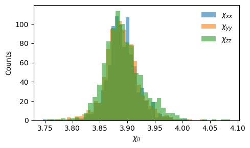
Dielectric to susceptibility: the electric susceptibility is related to the dielectric tensor by \(\boldsymbol{\chi} = \boldsymbol{\varepsilon} - \mathbf{I}\). For BaZrO\(_3\) at ambient conditions, the diagonal components of \(\boldsymbol{\chi}\) are around 4 while the off-diagonal components are close to zero for a cubic structure at equilibrium.

Normalization: GPUMD treats the pol field as an extensive (additive) quantity and normalizes it internally by the number of atoms, just as it normalizes energies and virials. For a finite system (polarizability), this convention is natural. For an extended system like BaZrO\(_3\), the susceptibility \(\boldsymbol{\chi}\) does not scale with system size, so the input must be multiplied by \(N\) to counteract the internal normalization:

s.info['pol'] = chi.flatten() * len(s)

During production MD simulations, GPUMD writes values that scale with system size (proportional to \(N\)) to polarizability.out; to recover the cell susceptibility \(\boldsymbol{\chi}\), the output must be divided by \(N\).

from ase.db import connect
import numpy as np

db = connect('barium-zirconate-susceptibility/reference-data.db')
structures = []
for row in db.select():
    s = row.toatoms()
    chi = np.array(row.data['dielectric']) - np.eye(3)
    s.info['pol'] = chi.flatten() * len(s)
    structures.append(s)
print(f'{len(structures)} structures prepared')

940 structures prepared

We can inspect the distribution of the diagonal susceptibility components:

import numpy as np
import matplotlib.pyplot as plt

chi_diag = np.array([
    s.info['pol'].reshape(3, 3).diagonal() / len(s)
    for s in structures
])

fig, ax = plt.subplots(figsize=(5, 3))
labels = [r'$\chi_{xx}$', r'$\chi_{yy}$', r'$\chi_{zz}$']
for i, lbl in enumerate(labels):
    ax.hist(chi_diag[:, i], bins=40, alpha=0.6, label=lbl)
ax.set_xlabel(r'$\chi_{ii}$')
ax.set_ylabel('Counts')
ax.legend(frameon=False)
fig.tight_layout()

Preparing training

We use setup_training to prepare the GPUMD input files. The key parameter is model_type=2, which instructs the nep executable to train a rank-2 TNEP model. The training uses a bagging ensemble with 5 splits: each split trains on 90% of the structures and evaluates on the remaining 10%, providing an estimate of model uncertainty.

Note that lambda_1 and lambda_2 are set to 0.002, well below the GPUMD default of 0.05. For TNEP models the output quantities (susceptibility tensor components) are typically much smaller in magnitude than energies and forces, so the default regularization strength over-regularizes the tensor outputs and leads to underfitting; smaller values are therefore recommended. For an analysis of the effect of regularization on TNEP models see Figure S13 of the Supporting Information in Xu et al. (2024).

Please refer to the GPUMD documentation for a full description of the training parameters.

import warnings
warnings.filterwarnings(
    'ignore',
    message='Failed to retrieve stresses for structure',
)

from calorine.nep import setup_training

parameters = dict(
    version=4,
    type=[3, 'Ba', 'Zr', 'O'],
    model_type=2,
    cutoff=[6, 4],
    n_max=[4, 4],
    basis_size=[10, 10],
    l_max=[4, 2],
    neuron=20,
    population=80,
    lambda_1=0.002,
    lambda_2=0.002,
    generation=200000,
    batch=500,
)

setup_training(
    parameters, structures,
    rootdir='barium-zirconate-susceptibility', overwrite=True,
    mode='bagging', n_splits=5, train_fraction=0.9,
)

The cell above prepares input files in barium-zirconate-susceptibility/nepmodel_full and five split directories nepmodel_split1 through nepmodel_split5. Training must be run in each directory by executing nep (the GPUMD training binary). Training the full model on 4× NVIDIA GH200 GPUs takes approximately 77 minutes (4602 s).

Pre-computed output from training on the full dataset and the five splits is available in barium-zirconate-susceptibility/example-output/ and is used in the analysis below.

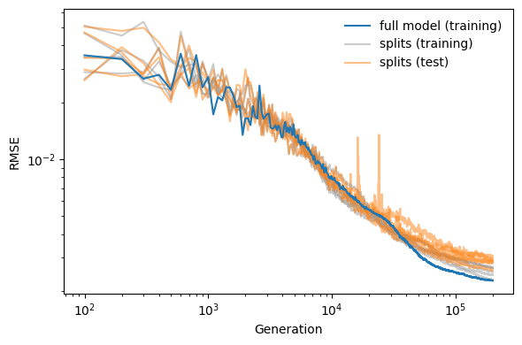
Analysis of the model

We can now analyze the convergence and accuracy of the full model.

from glob import glob
from calorine.nep import read_loss
import matplotlib.pyplot as plt

fig, ax = plt.subplots(figsize=(6, 4))

loss = read_loss('barium-zirconate-susceptibility/example-output/nepmodel_full/loss.out')
ax.plot(loss.RMSE_P_train, color='C0', zorder=100,
        label='full model (training)')

for fname in sorted(
    glob('barium-zirconate-susceptibility/example-output/nepmodel_split*/loss.out')
):
    loss = read_loss(fname)
    is_first = 'split1' in fname
    ax.plot(loss.RMSE_P_train, color='0.6', alpha=0.5,
            label='splits (training)' if is_first else '')
    ax.plot(loss.RMSE_P_test, color='C1', alpha=0.5,
            label='splits (test)' if is_first else '')

ax.set_xlabel('Generation')
ax.set_ylabel('RMSE')
ax.set_xscale('log')
ax.set_yscale('log')
ax.legend(frameon=False)
fig.tight_layout()

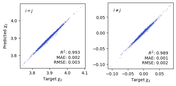
The parity plots below compare predicted and target susceptibility components for the training set. The diagonal components (\(i = j\)) and off-diagonal components (\(i \neq j\)) are shown separately; the latter are expected to be close to zero for a cubic structure at equilibrium. The coefficient of determination \(R^2\), mean absolute error (MAE), and root-mean-square error (RMSE) are shown in each panel.

import numpy as np
import matplotlib.pyplot as plt
from calorine.nep import get_parity_data, read_structures
from matplotlib import colormaps
from sklearn.metrics import (
    root_mean_squared_error,
    r2_score,
    mean_absolute_error,
)

example_dir = 'barium-zirconate-susceptibility/example-output'
structures_out, _ = read_structures(
    f'{example_dir}/nepmodel_full'
)

fig, axes = plt.subplots(figsize=(6, 3), ncols=2)
cmap = colormaps['coolwarm']

for k, (label, sel) in enumerate([
    (r'$i = j$', ['xx', 'yy', 'zz']),
    (r'$i \neq j$', ['yz', 'xz', 'xy']),
]):
    df = get_parity_data(
        structures_out, 'polarizability', selection=sel
    )
    err = df.target - df.predicted
    err /= np.max(np.abs(err))
    ax = axes[k]
    ax.scatter(df.target, df.predicted,
               s=3, alpha=0.2, color=cmap(err))
    ax.set_aspect('equal')
    ax.set_xlabel(r'Target $\chi_{ij}$')
    ax.text(0.08, 0.87, label, transform=ax.transAxes)
    r2 = r2_score(df.target, df.predicted)
    mae = mean_absolute_error(df.target, df.predicted)
    rmse = root_mean_squared_error(df.target, df.predicted)
    ax.text(
        0.92, 0.07,
        f'$R^2$: {r2:.3f}\nMAE: {mae:.3f}\nRMSE: {rmse:.3f}',
        ha='right', transform=ax.transAxes,
    )

axes[0].set_ylabel(r'Predicted $\chi_{ij}$')
fig.tight_layout()

Predicting the Raman spectrum

With trained TNEP models for the susceptibility, the Raman spectrum can be predicted from an NVE molecular dynamics trajectory. See the Predicting Raman spectra tutorial for a complete walkthrough using the BaZrO\(_3\) models trained here.