Dielectric functions

This tutorial demonstrates how to compute the dielectric function tensor \(\epsilon^{\alpha\beta}(\omega) = \epsilon_1^{\alpha\beta}(\omega) + i \epsilon_2^{\alpha\beta}(\omega)\) from a GPUMD molecular-dynamics simulation. GPUMD writes the time derivative of the polarization \(\dot{\mathbf{P}}(t)\) to a file named dpdt.out when using a qNEP model. The imaginary part of the dielectric tensor \(\epsilon_2^{\alpha\beta}(\omega)\) is related to the power spectral density of \(\dot{P}_\alpha(t)\) via

\[\epsilon_2^{\alpha\beta}(\omega) = \frac{1}{\epsilon_0 V k_\mathrm{B} T}\, \int_0^\infty \langle \dot{P}_\alpha(0)\,\dot{P}_\beta(\tau) \rangle\, e^{-i\omega\tau}\, d\tau,\]

where \(V\) is the simulation cell volume, \(T\) is the temperature, and \(\epsilon_0\) is the permittivity of free space. The isotropic average \(\bar{\epsilon}_2(\omega) = \frac{1}{3}\sum_\alpha \epsilon_2^{\alpha\alpha}(\omega)\) reduces to the scalar dielectric function for cubic or isotropic systems. The real part \(\epsilon_1^{\alpha\beta}(\omega)\) is obtained component-wise via the Kramers-Kronig relation

\[\epsilon_1^{\alpha\beta}(\omega) = \frac{2}{\pi}\, \mathcal{P}\int_0^\infty \frac{\omega'\,\epsilon_2^{\alpha\beta}(\omega')}{\omega'^2 - \omega^2}\, d\omega'.\]

The example data are from qNEP simulations of BaTiO\(_3\) at 100, 331, and 450 K from Z. Fan et al., J. Chem. Theory Comput. 22, 4787 (2026).

base = 'https://zenodo.org/records/20648097/files'
for T in [100, 331, 450]:
    fname = f'dpdt-BaTiO3-{T}K.txt'
    import os, urllib.request
    if not os.path.exists(fname):
        urllib.request.urlretrieve(f'{base}/{fname}', fname)
        print(f'Downloaded {fname}')
    else:
        print(f'{fname} already present')

dpdt-BaTiO3-100K.txt already present
dpdt-BaTiO3-331K.txt already present
dpdt-BaTiO3-450K.txt already present

Reading the data

The read_dpdt function reads a dpdt.out file into a pandas.DataFrame. The columns dPx, dPy, dPz are the Cartesian components of \(\dot{\mathbf{P}}(t)\) in units of \(e\)Å/fs, and Px, Py, Pz are the corresponding polarization components in units of \(e\)Å. The time step is read directly from the time column as the difference between consecutive rows.

from calorine.gpumd import read_dpdt

temperatures = [100, 331, 450]  # K
dfs_raw = {T: read_dpdt(f'dpdt-BaTiO3-{T}K.txt') for T in temperatures}

dfs_raw[450].head()

	time	dPx	dPy	dPz	Px	Py	Pz
0	0.02	-3.06855	-1.117540	1.867190	-61.3709	-22.3507	37.3438
1	0.04	-5.94163	0.009431	1.536860	-180.2030	-22.1621	68.0809
2	0.06	-5.86222	-2.869390	0.291382	-297.4480	-79.5499	73.9085
3	0.08	-4.57303	-4.939870	0.963120	-388.9080	-178.3470	93.1709
4	0.10	-1.08819	-5.468230	-0.305113	-410.6720	-287.7120	87.0687

Computing the dielectric function

get_dielectric_function computes both parts of the dielectric tensor from all three Cartesian components of \(\dot{\mathbf{P}}(t)\), returning the six unique Voigt components of the imaginary part \(\epsilon_2^{\alpha\beta}(\omega)\) together with the real part \(\epsilon_1^{\alpha\beta}(\omega)\) obtained via the Kramers-Kronig relation. The required physical parameters are

• volume: the simulation cell volume in Å\(^3\),

• temperature: the temperature in K.

The keyword column='dP' (the default) selects the dPx/dPy/dPz columns from read_dpdt. The time step is extracted automatically from the time column. The optional parameter t_sigma sets the width of a Gaussian window applied to the autocorrelation function before the Fourier transform (in ps); smaller values produce smoother spectra while larger values yield sharper features.

%%time
import numpy as np
from calorine.tools import get_dielectric_function

t_sigma = 2  # Gaussian window width in ps; smaller values give smoother spectra

lattice = np.array([[81.047018,  0.023688, -0.017573],
                    [ 0.014659, 80.976750, -0.016819],
                    [-0.017772, -0.026703, 80.939036]])
volume = np.abs(np.linalg.det(lattice))  # Angstrom^3
print(f'Cell volume: {volume:.1f} Angstrom^3')

dfs = {}
for T in temperatures:
    dfs[T] = get_dielectric_function(dfs_raw[T], volume, T, column='dP', t_sigma=t_sigma)
dfs[450].head()

Cell volume: 531196.7 Angstrom^3
CPU times: user 1min 47s, sys: 14.8 s, total: 2min 2s
Wall time: 1min

	angular_frequency	wavenumber_invcm	epsilon_imag_xx	epsilon_imag_yy	epsilon_imag_zz	epsilon_imag_yz	epsilon_imag_xz	epsilon_imag_xy	conductivity_xx	conductivity_yy	conductivity_zz	conductivity_yz	conductivity_xz	conductivity_xy	epsilon_real_xx	epsilon_real_yy	epsilon_real_zz	epsilon_real_yz	epsilon_real_xz	epsilon_real_xy
0	0.006283	0.033357	124255.284323	59899.173855	41507.546044	-1965.406627	-6210.587144	7150.681630	6912.770709	3332.407606	2309.214856	-109.342677	-345.517417	397.818272	62862.620438	31549.732382	22417.644882	-946.858042	-2967.715355	3434.593445
1	0.012567	0.066714	62149.270547	29962.758741	20763.426580	-982.586187	-3105.680122	3575.548379	6915.177239	3333.873197	2310.288981	-109.329644	-345.560427	397.841367	31555.872535	16458.496943	11960.202017	-451.554422	-1402.762191	1632.702157
2	0.018850	0.100071	41456.876064	19989.807161	13853.010279	-654.927121	-2070.882673	2383.929419	6919.187705	3336.315735	2312.079141	-109.307891	-345.632071	397.879838	15076.692173	8514.590987	6455.453043	-190.875112	-579.063694	684.318563
3	0.025133	0.133428	31117.883584	15007.720701	10401.019451	-491.058181	-1553.612344	1788.188890	6924.801479	3339.735051	2314.585267	-109.277368	-345.732287	397.933652	9885.493452	6012.157721	4721.399918	-108.756631	-319.587462	385.573541
4	0.031417	0.166785	24920.248748	12021.979431	8332.398456	-392.705044	-1243.352559	1430.799575	6932.017682	3344.130904	2317.807258	-109.238007	-345.860991	398.002767	7561.505183	4891.890736	3945.128978	-71.994153	-203.428301	251.844760

Kramers-Kronig integration method

The Kramers-Kronig step is performed internally by get_dielectric_function (controlled by return_real_part, which defaults to True). Two integration methods are available via the kk_method keyword:

• 'vectorized' (default): exact trapezoid rule, \(\mathcal{O}(n^2)\) time and memory.

• 'fft': \(\mathcal{O}(n \log n)\) Hilbert-transform approximation; faster for large arrays but can deviate near sharp features.

The section below compares both methods on the 100 K data, which has the sharpest phonon peaks and provides the most stringent test.

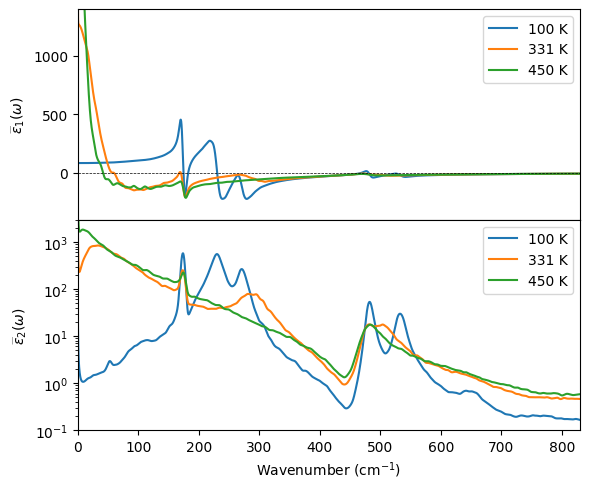
Visualization

import matplotlib.pyplot as plt

def isotropic_average(df, prefix):
    return (df[f'{prefix}_xx'] + df[f'{prefix}_yy'] + df[f'{prefix}_zz']) / 3


fig, (ax1, ax2) = plt.subplots(2, 1, figsize=(6, 5), sharex=True)

for T in temperatures:
    df = dfs[T]
    ax1.plot(df.wavenumber_invcm, isotropic_average(df, 'epsilon_real'), label=f'{T} K')
    ax2.plot(df.wavenumber_invcm, isotropic_average(df, 'epsilon_imag'), label=f'{T} K')

ax1.axhline(0, color='k', linewidth=0.5, linestyle='--')
ax1.set_ylabel(r'$\widebar{\epsilon}_1(\omega)$')
ax1.legend()
ax1.set_xlim(0, 830)
ax1.set_ylim(-400, 1400)

ax2.set_xlabel(r'Wavenumber (cm$^{-1}$)')
ax2.set_ylabel(r'$\widebar{\epsilon}_2(\omega)$')
ax2.legend()
ax2.set_yscale('log')
ax2.set_ylim(0.1, 3e3)

fig.tight_layout()
fig.subplots_adjust(hspace=0)

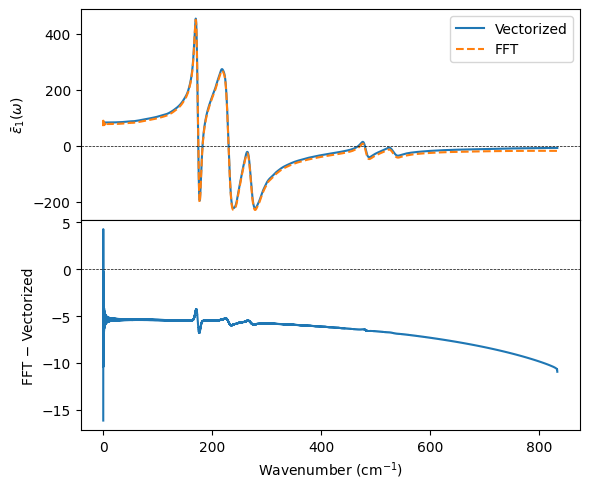
Accuracy: FFT vs. vectorized

dfs[100] was computed with the default kk_method='vectorized'. The cell below recomputes the 100 K spectrum with kk_method='fft' for comparison. The two methods agree well across most of the spectrum, but the FFT approximation can deviate near sharp features and at larger frequencies.

df_vec = dfs[100].iloc[5:]
df_fft = get_dielectric_function(dfs_raw[100], volume, 100,
                                 column='dP', t_sigma=t_sigma, kk_method='fft').iloc[5:]

fig, (ax1, ax2) = plt.subplots(2, 1, figsize=(6, 5), sharex=True)

ax1.plot(df_vec.wavenumber_invcm, isotropic_average(df_vec, 'epsilon_real'), label='Vectorized')
ax1.plot(df_fft.wavenumber_invcm, isotropic_average(df_fft, 'epsilon_real'), '--', label='FFT')
ax1.axhline(0, color='k', linewidth=0.5, linestyle='--')
ax1.set_ylabel(r'$\bar{\epsilon}_1(\omega)$')
ax1.legend()

diff = isotropic_average(df_fft, 'epsilon_real').to_numpy() - isotropic_average(df_vec, 'epsilon_real').to_numpy()
ax2.plot(df_vec.wavenumber_invcm, diff)
ax2.axhline(0, color='k', linewidth=0.5, linestyle='--')
ax2.set_xlabel(r'Wavenumber (cm$^{-1}$)')
ax2.set_ylabel('FFT − Vectorized')

fig.tight_layout()
fig.subplots_adjust(hspace=0)

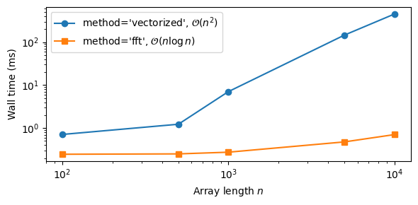
Kramers-Kronig performance

The timing comparison below illustrates the performance advantage of the 'fft' method over the 'vectorized' approach, which comes at a small cost in accuracy (see above).

from calorine.tools import apply_kramers_kronig
import time
from pandas import DataFrame

sizes = [100, 500, 1000, 5000, 10000]
times_vec = []
times_fft = []

for n in sizes:
    df_test = DataFrame({'angular_frequency': np.linspace(0.1, 100.0, n),
                         'epsilon_imag': np.sin(np.linspace(0.1, 100.0, n))})

    nrep = max(3, 200 // n)
    t0 = time.perf_counter()
    for _ in range(nrep):
        apply_kramers_kronig(df_test, method='vectorized')
    times_vec.append((time.perf_counter() - t0) / nrep * 1000)

    t0 = time.perf_counter()
    for _ in range(500):
        apply_kramers_kronig(df_test, method='fft')
    times_fft.append((time.perf_counter() - t0) / 500 * 1000)

fig, ax = plt.subplots(figsize=(6, 3))
ax.loglog(sizes, times_vec, 'o-', label=r"method='vectorized', $\mathcal{O}(n^2)$")
ax.loglog(sizes, times_fft, 's-', label=r"method='fft', $\mathcal{O}(n \log n)$")
ax.set_xlabel('Array length $n$')
ax.set_ylabel('Wall time (ms)')
ax.legend()
fig.tight_layout()