Modifying and extending NEP models#

A trained NEP model can serve as the starting point for further development rather than as a final product. Common workflows include:

Increasing capacity: expand the number of neurons or add higher-body descriptor terms when the initial architecture turns out to be too small.
Adding a charge output: promote a plain potential model to a charge-aware qNEP model by attaching a charge output head, then continue training with charge targets.
Species manipulation: prune a multi-element model down to a subset of elements, or extend an existing model with a new species without discarding the learned potential surface.
Reducing capacity: remove neurons or descriptor terms that contribute little to accuracy, for faster inference or as a starting point for fine-tuning on a narrower dataset.

calorine provides five Model methods for these use cases:

Method	What it does	Retraining required?
`augment()`	Expand neurons, descriptors, or add a charge head	Yes
`prune()`	Reduce neurons, remove descriptor terms, or drop the charge head	Yes
`remove_species()`	Remove one or more species	No (optional)
`keep_species()`	Retain a subset of species, dropping all others	No (optional)
`add_species()`	Add one or more species	Yes

All methods return a new Model instance; the source model is never modified in place.

[1]:

import numpy as np
import matplotlib.pyplot as plt
from calorine.nep import read_model

Loading a model#

The modification methods require the SNES restart file to be loaded alongside the model. The restart file stores a mean mu and a standard deviation sigma for every parameter; these are the current estimate of the SNES optimizer of the optimal value and exploration width, respectively.

[2]:

model = read_model('../tests/nep_models/nep4_PbTe.txt',
                   restart_file='../tests/nep_models/nep4_PbTe.restart')
display(model)

Field	Value
version	4
model_type	potential
types	('Te', 'Pb')
radial_cutoff	8.0
angular_cutoff	4.0
n_basis_radial	8
n_basis_angular	8
n_max_radial	4
n_max_angular	4
l_max_3b	4
l_max_4b	2
l_max_5b	0
has_q_112	0
has_q_123	0
has_q_233	0
has_q_134	0
n_descriptor_radial	5
n_descriptor_angular	25
n_neuron	30
n_parameters	2311
n_descriptor_parameters	360
n_ann_parameters	1921
sqrt_epsilon_infinity	None
restart_parameters	available
zbl	None
zbl_typewise_cutoff_factor	None
max_neighbors_radial	74
max_neighbors_angular	10
radial_typewise_cutoff_factor	None
angular_typewise_cutoff_factor	None
Dimension of ann_parameters	(2, 3)
Dimension of q_scaler	30
Dimension of radial_descriptor_weights	(5, 9)
Dimension of angular_descriptor_weights	(5, 9)

Expanding a model with `augment()`#

augment() applies one or more structural changes atomically and returns a new model. All changes can be combined in a single call.

Initialization of new and existing parameters#

After a successful training run, many sigma values in the restart file are near zero — parameters that SNES drove toward zero are effectively dormant and should stay that way. augment() handles the restart as follows:

Existing parameters: mu is copied verbatim (trained values preserved); sigma is re-opened to max(sigma_floor, sigma_factor × |mu|), proportional to each parameter’s magnitude. Near-zero parameters remain dormant; active ones can adapt.
New parameters: mu = 0, sigma = sigma_new. When training with nep they will be started silently and the optimization will discover their values from scratch.

Adding neurons#

[3]:

larger = model.augment(n_neuron=40)

print(f'n_neuron     : {model.n_neuron} -> {larger.n_neuron}')
print(f'n_parameters : {model.n_parameters} -> {larger.n_parameters}')

# The source model is unmodified
assert model.n_neuron == 30

n_neuron     : 30 -> 40
n_parameters : 2311 -> 2951

Adding descriptor terms#

The 4-body and 5-body descriptor terms are controlled by l_max_4b, l_max_5b, and the has_q_* flags. Enabling a new body-order term adds n_max_angular + 1 new descriptor dimensions and the corresponding columns in the input-layer weight matrix w0.

[4]:

print(f'Before: l_max_5b = {model.l_max_5b}, '
      f'n_descriptor_angular = {model.n_descriptor_angular}')

with_5b = model.augment(l_max_5b=1)

print(f'After:  l_max_5b = {with_5b.l_max_5b}, '
      f'n_descriptor_angular = {with_5b.n_descriptor_angular}')
print(f'Δ = {with_5b.n_descriptor_angular - model.n_descriptor_angular} '
      f'= n_max_angular + 1 = {model.n_max_angular + 1}')

Before: l_max_5b = 0, n_descriptor_angular = 25
After:  l_max_5b = 1, n_descriptor_angular = 30
Δ = 5 = n_max_angular + 1 = 5

Adding a charge output head#

Setting charge_head=True promotes a plain NEP model (potential) to a charge-aware qNEP model (potential_with_charges). A second output node is added per species (the charge head) and sqrt_epsilon_infinity is initialized to one (ε∞ = 1, the vacuum value). The charge weights w1_charge start at zero, so the charge contribution is silent at the start of training.

[5]:

charge_model = model.augment(charge_head=True)

print(f'model_type   : {model.model_type!r} -> {charge_model.model_type!r}')
print(f'n_parameters : {model.n_parameters} -> {charge_model.n_parameters}')

model_type   : 'potential' -> 'potential_with_charges'
n_parameters : 2311 -> 2372

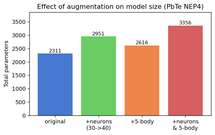
Combining augmentations#

All changes can be requested in a single call. The new w0 matrix grows in both dimensions simultaneously, so combining neuron expansion with descriptor expansion is equivalent to doing them atomically.

[6]:

aug = model.augment(n_neuron=40, l_max_5b=1)

labels = ['original', '+neurons\n(30->40)', '+5-body', '+neurons\n& 5-body']
counts = [model.n_parameters, larger.n_parameters,
          with_5b.n_parameters, aug.n_parameters]

fig, ax = plt.subplots(figsize=(5.5, 3.5), dpi=130)
bars = ax.bar(labels, counts, color=['#4878d0', '#6acc65', '#ee854a', '#d65f5f'])
ax.set_ylabel('Total parameters')
ax.set_title('Effect of augmentation on model size (PbTe NEP4)')
for bar, c in zip(bars, counts):
    ax.text(bar.get_x() + bar.get_width() / 2, c + 5, str(c),
            ha='center', va='bottom', fontsize=9)
ax.set_ylim(0, max(counts) * 1.15)
fig.tight_layout()
plt.show()

../_images/get_started_modifying_models_11_0.png

Writing the augmented model to disk#

The augmented model is written with the same write() / write_restart() methods used for any model. The resulting nep.txt and nep.restart files can be placed directly in a GPUMD working directory to resume training.

[7]:

aug.write('nep.txt')
aug.write_restart('nep.restart')

Before starting a new training run with the augmented model, nep.in must be updated to reflect the new architecture. GPUMD reads nep.in — not nep.txt — to determine the model size and compute how many values to read from nep.restart. Using a stale nep.in causes a stride mismatch: GPUMD reads the restart file with the old parameter count and all values beyond the first mismatch are garbage, producing training-from-scratch-level initial loss even when sigma is zero.

training_parameters returns the architecture fields in the format accepted by write_nepfile():

[8]:

print(aug.training_parameters)

{'version': 4, 'type': [2, 'Te', 'Pb'], 'cutoff': [8.0, 4.0], 'n_max': [4, 4], 'basis_size': [8, 8], 'l_max': [4, 2, 1], 'neuron': 40}

To update an existing nep.in with the new architecture while keeping the training-specific settings, merge training_parameters into the existing parameter dict and write the result.

[9]:

from calorine.nep import read_nepfile, write_nepfile

params = read_nepfile('nep-PbTe.in')  # read the old nep.in file
params.update(aug.training_parameters)
write_nepfile(params, '.')
print(open('nep.in').read())

version  4
type  2 Te Pb
cutoff  8.0 4.0
n_max  4 4
basis_size  8 8
l_max  4 2 1
neuron  40
generation  100000
batch  1000
lambda_e  1.0
lambda_f  1.0
lambda_v  0.1

Removing species with `remove_species()`#

remove_species() prunes all parameters associated with the listed elements, i.e., the ANN sub-networks, descriptor weight pairs, and (if the restart is loaded) their SNES statistics. A common use case is extracting a single-element model from a multi-element potential.

[10]:

te_only = model.remove_species(['Pb'])

print(f'Original types : {model.types}')
print(f'Retained types : {te_only.types}')
print()
print(f'n_parameters   : {model.n_parameters} -> {te_only.n_parameters}')

# Source model is unchanged
assert model.types == ('Te', 'Pb')

Original types : ('Te', 'Pb')
Retained types : ('Te',)

n_parameters   : 2311 -> 1081

When restart_parameters are loaded, the surviving parameters also receive adaptive sigma values (same sigma_factor / sigma_floor scheme as augment()), re-opening the SNES search distribution for the next training run.

Retaining species with `keep_species()`#

When isolating a small subset from a large foundation model, listing every species to drop via remove_species() is impractical. keep_species() accepts the elements to retain and derives the removal list automatically.

[11]:

# Isolate Te from the binary model — equivalent to remove_species(['Pb'])
te_model = model.keep_species(['Te'])

print(f'Original types : {model.types}')
print(f'Retained types : {te_model.types}')
print(f'n_parameters   : {model.n_parameters} -> {te_model.n_parameters}')

Original types : ('Te', 'Pb')
Retained types : ('Te',)
n_parameters   : 2311 -> 1081

Adding species with `add_species()`#

add_species() extends the model with:

A new per-species ANN sub-network (for each added element)
All new (species_1, species_2) descriptor weight pairs involving the new elements

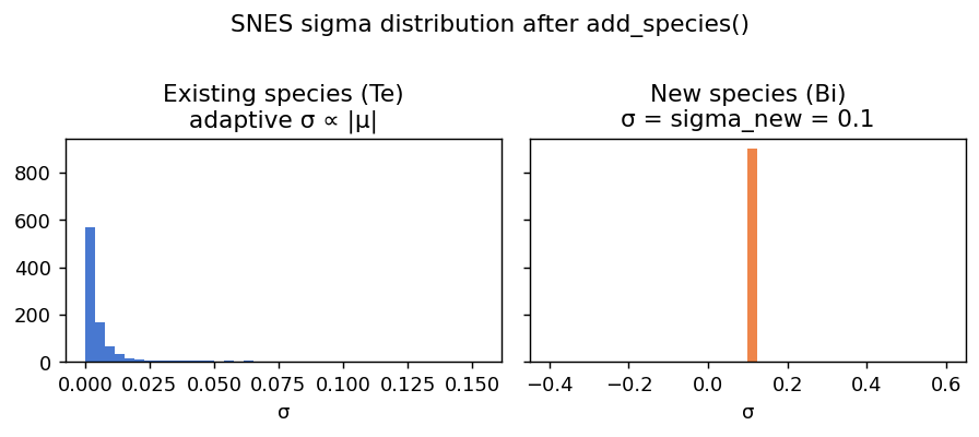
All new parameters are initialized with mu drawn uniformly from [-1, 1] (matching GPUMD’s fresh-model initialization) and sigma = sigma_new. The existing species retain their trained weights and receive fresh SNES sigma values.

Because the new parameters start at zero, the model must be trained further before the new element is meaningful.

[12]:

extended = model.add_species(['Bi'])

print(f'Types         : {model.types} -> {extended.types}')
print(f'n_parameters  : {model.n_parameters} -> {extended.n_parameters}')
print()
# New sub-network: mu drawn uniformly from [-1, 1]
bi_w0 = extended.ann_parameters['Bi']['w0']
print(f'Bi w0 shape   : {bi_w0.shape}')
print(f'Bi w0 range   : [{bi_w0.min():.3f}, {bi_w0.max():.3f}]')

# All new descriptor pairs are present
new_pairs = [(s1, s2) for s1 in extended.types for s2 in extended.types
             if 'Bi' in (s1, s2)]
print(f'New descriptor pairs: {new_pairs}')

Types         : ('Te', 'Pb') -> ('Te', 'Pb', 'Bi')
n_parameters  : 2311 -> 3721

Bi w0 shape   : (30, 30)
Bi w0 range   : [-0.998, 0.999]
New descriptor pairs: [('Te', 'Bi'), ('Pb', 'Bi'), ('Bi', 'Te'), ('Bi', 'Pb'), ('Bi', 'Bi')]

[13]:

sigma_new_val = 0.1    # default value (matches GPUMD sigma0)

bi_sigma_w0 = extended.restart_parameters['ann_sigma']['Bi']['w0']
te_mu_w0    = model.restart_parameters['ann_mu']['Te']['w0']
te_sigma_w0 = extended.restart_parameters['ann_sigma']['Te']['w0']

fig, axes = plt.subplots(1, 2, figsize=(7, 3), dpi=130, sharey=True)
axes[0].hist(te_sigma_w0.flatten(), bins=40, color='#4878d0')
axes[0].set_title('Existing species (Te)\nadaptive σ ∝ |μ|')
axes[0].set_xlabel('σ')
axes[1].hist(bi_sigma_w0.flatten(), bins=40, color='#ee854a')
axes[1].set_title(f'New species (Bi)\nσ = sigma_new = {sigma_new_val}')
axes[1].set_xlabel('σ')
fig.suptitle('SNES sigma distribution after add_species()', y=1.01)
fig.tight_layout()

../_images/get_started_modifying_models_25_0.png

Pruning with `prune()`#

prune() is the complement to augment(): it returns a new model with a smaller architecture. All surviving parameters receive adaptive SNES sigma, max(sigma_floor, sigma_factor × |μ|), so the optimizer can adapt from the reduced starting point.

Reducing neurons#

When n_neuron is reduced, neurons are ranked by their importance score averaged over species:

\[\text{importance}[n] = \frac{1}{|S|} \sum_s \lVert w^{(0)}_{s}[n, :] \rVert_2 \times |w^{(1)}_{s}[n]|\]

For charge models, \(|w^{(1)}_{s}[n]|\) is replaced by \(|w^{(1)}_{s}[n]| + |w^{(1,\mathrm{charge})}_{s}[n]|\). The top-scoring neurons are kept; the rest are discarded.

[14]:

pruned_neurons = model.prune(n_neuron=20)

print(f'Original : n_neuron={model.n_neuron}, n_parameters={model.n_parameters}')
print(f'Pruned   : n_neuron={pruned_neurons.n_neuron}, n_parameters={pruned_neurons.n_parameters}')

# Source model is unmodified
assert model.n_neuron == 30

Original : n_neuron=30, n_parameters=2311
Pruned   : n_neuron=20, n_parameters=1671

Removing descriptor terms#

Setting l_max_4b=0 (or has_q_112=False, etc.) drops the corresponding descriptor columns entirely, reducing n_descriptor_angular and n_parameters.

Note: reducing l_max_4b to a non-zero value (e.g. 3 → 2) only changes the header — the descriptor dimensions are unchanged because the same number of (n_max_angular + 1) columns is stored for any non-zero l_max_4b.

[15]:

pruned_desc = model.prune(l_max_4b=0)

n_removed = model.n_descriptor_angular - pruned_desc.n_descriptor_angular
print(f'Original : l_max_4b={model.l_max_4b}, n_descriptor_angular={model.n_descriptor_angular}')
print(f'Pruned   : l_max_4b={pruned_desc.l_max_4b}, n_descriptor_angular={pruned_desc.n_descriptor_angular}')
print(f'Columns removed: {n_removed} (= n_max_angular + 1 = {model.n_max_angular + 1})')

Original : l_max_4b=2, n_descriptor_angular=25
Pruned   : l_max_4b=0, n_descriptor_angular=20
Columns removed: 5 (= n_max_angular + 1 = 5)

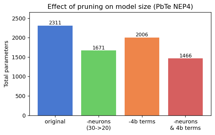
Combining reductions#

Both axes can be combined in a single call, just like augment().

[16]:

pruned = model.prune(n_neuron=20, l_max_4b=0)

labels = ['original', '-neurons\n(30->20)', '-4b terms', '-neurons\n& 4b terms']
counts = [model.n_parameters, pruned_neurons.n_parameters,
          pruned_desc.n_parameters, pruned.n_parameters]

fig, ax = plt.subplots(figsize=(5.5, 3.5), dpi=130)
bars = ax.bar(labels, counts, color=['#4878d0', '#6acc65', '#ee854a', '#d65f5f'])
ax.set_ylabel('Total parameters')
ax.set_title('Effect of pruning on model size (PbTe NEP4)')
for bar, c in zip(bars, counts):
    ax.text(bar.get_x() + bar.get_width() / 2, c + 5, str(c),
            ha='center', va='bottom', fontsize=9)
ax.set_ylim(0, max(counts) * 1.15)
fig.tight_layout()
plt.show()

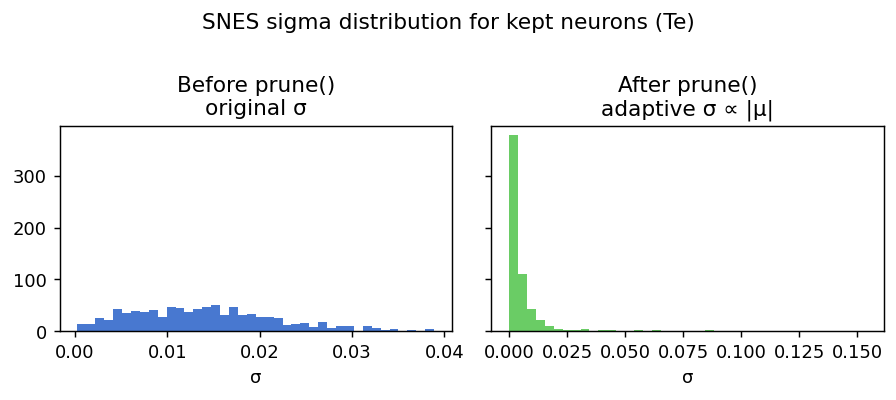
../_images/get_started_modifying_models_31_0.png

Initialization of surviving parameters#

Surviving parameters receive adaptive SNES sigma: sigma = max(sigma_floor, sigma_factor × |μ|). This is the same scheme applied to existing parameters in augment() and add_species() — parameters with large trained values get more room to adapt, while near-zero parameters remain dormant.

[17]:

sigma_factor_val = 0.1   # default

s = 'Te'
mu_w0 = model.restart_parameters['ann_mu'][s]['w0']
sigma_w0_before = model.restart_parameters['ann_sigma'][s]['w0']
sigma_w0_after = pruned_neurons.restart_parameters['ann_sigma'][s]['w0']

fig, axes = plt.subplots(1, 2, figsize=(7, 3), dpi=130, sharey=True)
axes[0].hist(sigma_w0_before.flatten(), bins=40, color='#4878d0')
axes[0].set_title(f'Before prune()\noriginal σ')
axes[0].set_xlabel('σ')
axes[1].hist(sigma_w0_after.flatten(), bins=40, color='#6acc65')
axes[1].set_title(f'After prune()\nadaptive σ ∝ |μ|')
axes[1].set_xlabel('σ')
fig.suptitle(f'SNES sigma distribution for kept neurons ({s})', y=1.01)
fig.tight_layout()

../_images/get_started_modifying_models_33_0.png

Composing operations#

Each method returns a new Model, so operations can be chained directly.

[18]:

# Swap Pb for Bi: prune Pb, then add Bi
swapped = model.remove_species(['Pb']).add_species(['Bi'])
print(f'Original : {model.types}')
print(f'Swapped  : {swapped.types}')

Original : ('Te', 'Pb')
Swapped  : ('Te', 'Bi')

[19]:

# Expand the architecture and add a new element in one pipeline
final = model.augment(n_neuron=40).add_species(['Bi'])
print(f'Types        : {final.types}')
print(f'n_neuron     : {final.n_neuron}')
print(f'n_parameters : {final.n_parameters}')

Types        : ('Te', 'Pb', 'Bi')
n_neuron     : 40
n_parameters : 4681

[20]:

# Trim to essentials, then add a new element
compact = model.prune(n_neuron=20, l_max_4b=0).add_species(['Bi'])
print(f'Types        : {compact.types}')
print(f'n_neuron     : {compact.n_neuron}')
print(f'n_parameters : {compact.n_parameters}')

Types        : ('Te', 'Pb', 'Bi')
n_neuron     : 20
n_parameters : 2456