Infrared spectra

Introduction

Infrared (IR) spectroscopy probes vibrational modes that change the electric polarization of a material. For a bulk liquid or solid, the imaginary part of the dielectric function \(\varepsilon_2(\omega)\) governs IR absorption and is related to the power spectral density of the time derivative of the macroscopic polarization \(\dot{\mathbf{P}}(t)\) via

\[\varepsilon_2(\omega) = \frac{1}{\varepsilon_0 V k_\mathrm{B} T} \int_0^\infty \langle \dot{P}(0)\,\dot{P}(t) \rangle\, e^{-i\omega t}\, dt,\]

where \(V\) is the simulation cell volume, \(T\) the temperature, and \(\varepsilon_0\) the permittivity of free space. In an MD simulation, \(\mathbf{P}(t)\) is the total cell dipole moment (the polarization); its time evolution is sampled at each step.

TNEP models extend the standard NEP framework with a rank-1 model that predicts \(\mathbf{P}(t)\) at every MD step. GPUMD writes the polarization time series to dipole.out when the keyword dump_dipole is present in run.in. The calorine function get_ir_spectrum reads this output and converts the autocorrelation function (ACF) of \(\mathbf{P}(t)\) to \(\varepsilon_2(\omega)\) via the Fourier transform using the identity

\[\mathrm{PSD}[\dot{P}(\omega)] = \omega^2\,\mathrm{PSD}[P(\omega)].\]

This tutorial uses bulk water simulated with the TNEP model of Xu et al., J. Chem. Theory Comput. 20, 3273 (2024). The simulated spectrum is compared with the experimental IR absorption spectrum from J.-J. Max and C. Chapados, J. Chem. Phys. 131, 184505 (2009).

See the TNEP polarization tutorial for how to train the type of polarization model used here, and the dielectric function tutorial for an analysis of the full dielectric tensor and Kramers-Kronig real part. The latter uses BaTiO\(_3\) for illustration and a qNEP model instead of the NEP+TNEP model approach taken here.

Simulation setup

The simulation uses two NEP models:

• nep_energy.txt — the PES (potential energy surface) model.

• nep_polarization.txt — the rank-1 polarization model (TNEP).

Both models are from the Zenodo record 10.5281/zenodo.10257363 (Xu et al. 2024). Note that on Zenodo the polarization model is named nep_dipole_bulk_water.txt — a misnomer for an extended-system polarization model. The nep4 header was updated to nep4_dipole for compatibility with newer GPUMD versions.

The simulation box contains 6,912 water molecules (20,736 atoms). The protocol is:

1. NPT equilibration: 100,000 steps × 0.5 fs = 50 ps at 300 K.

2. NVE production: 200,000 steps × 0.5 fs = 100 ps; dump_dipole 4 writes \(\mathbf{P}(t)\) every 4 × 0.5 fs = 2 fs, giving 50,000 frames in dipole.out.

potential nep_energy.txt
potential nep_polarization.txt
time_step 0.5
velocity 300

ensemble npt_scr 300 300 100 0 2 100
dump_thermo 400
dump_restart 20000
run 100000

ensemble nve
dump_thermo 400
dump_dipole 4
dump_restart 20000
run 200000

On a single NVIDIA GH200 GPU the complete simulation takes approximately 16 minutes (NPT equilibration approx. 5 min, NVE production approx. 11 min). Using the above settings, you can run the MD yourself, but you can also choose to download the trajectory from Zenodo by running the next cell.

import os
import zipfile
import urllib.request

url = 'https://zenodo.org/records/20679922/files/water-ir.zip'
if not os.path.exists('water-ir'):
    urllib.request.urlretrieve(url, 'water-ir.zip')
    with zipfile.ZipFile('water-ir.zip') as zf:
        zf.extractall('.')
    os.remove('water-ir.zip')
    print('Downloaded and extracted water-ir/')
else:
    print('water-ir/ already present')

water-ir/ already present

import numpy as np
from ase.io import read
from calorine.gpumd import read_dipole

atoms = read('water-ir/model.xyz')
volume = atoms.get_volume()  # Angstrom^3
print(f'Volume: {volume:.0f} ų  ({len(atoms)} atoms)')

dipole_df = read_dipole('water-ir/dipole.out')

# dt: dump_dipole 4 * time_step 0.5 fs = 2 fs = 0.002 ps
dt = 0.002   # ps
temperature = 300  # K
print(f'Frames: {len(dipole_df)}, dt = {dt} ps')

Volume: 193211 ų  (20736 atoms)
Frames: 50000, dt = 0.002 ps

Computing the IR spectrum

get_ir_spectrum computes \(\varepsilon_2(\omega)\) from the polarization time series \(\mathbf{P}(t)\). The required parameters are:

• volume: cell volume in ų (read from the structure file),

• temperature: temperature in K (300 K).

The keyword column='mu' selects the mu_x/mu_y/mu_z columns from the read_dipole output and indicates that the input is the polarization \(\mathbf{P}(t)\) itself rather than its time derivative; the \(\omega^2\) factor from the identity \(\mathrm{PSD}[\dot{P}] = \omega^2\,\mathrm{PSD}[P]\) is applied internally. Since dipole.out has no time column, dt must be passed explicitly (0.002 ps here, corresponding to dump_dipole 4 × time_step 0.5 fs).

The optional t_sigma parameter (in ps) controls the width of a Gaussian window applied to the ACF before the Fourier transform; smaller values give smoother spectra at the cost of frequency resolution.

The accessible frequency range is bounded at both ends. The lower cutoff is set by the NVE run length: the ACF is evaluated up to a maximum lag of \(T_\mathrm{ACF}\) (by default 25,% of the trajectory, giving 25 ps here), which limits the raw frequency resolution to \(\Delta\tilde{\nu} = 1/(c\,T_\mathrm{ACF}) \approx 1.3\,\mathrm{cm}^{-1}\). Gaussian window with t_sigma = 0.5 ps broadens spectral lines further to \(\sigma_{\tilde{\nu}} = 1/(2\pi c\,t_\sigma) \approx 11\,\mathrm{cm}^{-1}\) (FWHM \(\approx\) 25 cm\(^{-1}\)), so features below roughly 50 cm\(^{-1}\) are not reliably resolved with the current settings. Longer NVE runs lower this cutoff proportionally. The upper cutoff follows from the Nyquist criterion: the highest resolvable frequency is \(\tilde{\nu}_\mathrm{max} = 1/(2\,c\,\Delta t)\), where \(\Delta t\) is the polarization sampling interval (dump_dipole \(\times\) time_step). For \(\Delta t = 2\) fs this gives \(\tilde{\nu}_\mathrm{max} \approx 8300\,\mathrm{cm}^{-1}\), well above the OH-stretch band. A shorter sampling interval is required to access higher frequencies.

The statistical quality of the spectrum improves with simulation length. It can also be improved by averaging spectra from multiple independent NVE runs, which can be trivially parallelized.

from calorine.tools import get_ir_spectrum

ir_df = get_ir_spectrum(dipole_df, volume=volume, temperature=temperature,
                        column='mu', dt=dt, t_sigma=0.5)
ir_df.head()

	angular_frequency	wavenumber_invcm	epsilon_imag	conductivity
0	0.125669	0.667155	11.635935	12.947241
1	0.251337	1.334310	23.140200	51.495949
2	0.377006	2.001465	34.383646	114.775488
3	0.502675	2.668620	45.242099	201.362550
4	0.628344	3.335774	55.598677	309.321731

Quantum corrections

Classical MD samples the Boltzmann distribution and therefore underestimates spectral intensities at frequencies where \(\hbar\omega \gtrsim k_\mathrm{B}T\). At 300 K, \(k_\mathrm{B}T / h \approx 208\ \mathrm{cm}^{-1}\), so the correction is significant for the OH-stretch band (approx. 3400 cm\(^{-1}\)) but modest for the low-frequency libration and bending modes.

The first-order quantum correction factor (M. Cardona, Topics in Applied Physics, Vol. 50, Springer, 1982) is

\[f(\omega) = \frac{\beta\hbar\omega}{1 - e^{-\beta\hbar\omega}}, \qquad \beta = \frac{1}{k_\mathrm{B} T}.\]

apply_quantum_correction multiplies each spectral point by \(f(\omega)\) and returns the corrected spectrum in a new column epsilon_imag_qm.

from calorine.tools import apply_quantum_correction

ir_qm = apply_quantum_correction(
    ir_df, temperature, 'epsilon_imag', order='first')

Now we can plot the result.

import matplotlib.pyplot as plt

# Load experimental spectrum (Max & Chapados 2009)
exp_data = np.loadtxt('water-ir/ir_experiment_Max.txt')
wn_exp = exp_data[:, 0]
alpha_exp = exp_data[:, 1]

# Normalize to the OH-stretch peak (~3400 cm^-1) for comparison
wn = ir_df['wavenumber_invcm']
mask_oh = (wn > 3000) & (wn < 3800)
mask_oh_exp = (wn_exp > 3000) & (wn_exp < 3800)

scale_cl = ir_df.loc[mask_oh, 'epsilon_imag'].max()
scale_qm = ir_qm.loc[mask_oh, 'epsilon_imag_qm'].max()
scale_exp = alpha_exp[mask_oh_exp].max()

fig, ax = plt.subplots(figsize=(6, 4))
ax.plot(wn, ir_df['epsilon_imag'] / scale_cl, label='Classical MD')
ax.plot(wn, ir_qm['epsilon_imag_qm'] / scale_qm, label='Quantum corrected')
ax.plot(wn_exp, alpha_exp / scale_exp, 'k--', label='Experiment (Max 2009)')
ax.set_xlabel(r'Wavenumber (cm$^{-1}$)')
ax.set_ylabel('IR absorption (normalized)')
ax.set_xlim(50, 4500)
ax.set_ylim(0, 2.1)
ax.legend()
fig.tight_layout()

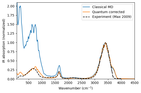
Agreement with experiment

The quantum-corrected spectrum reproduces the main spectral features of liquid water: the translational band near 150 cm\(^{-1}\) (attributed to translational motions of hydrogen-bonded molecules), the libration band (about 400–900 cm\(^{-1}\)), the bending mode (about 1600 cm\(^{-1}\)), and the OH-stretch band (about 3400 cm\(^{-1}\)).

The quantum correction applied here accounts for occupation statistics only — it rescales band intensities via the Bose-Einstein factor \(f(\omega) = \beta\hbar\omega / (1 - e^{-\beta\hbar\omega})\). Without this correction the classical spectrum strongly underestimates the intensity of the OH-stretch band relative to the lower-frequency bands. Quantum effects on vibrational frequencies (zero-point motion, tunnelling) are not captured by this correction; they can be addressed via thermostatted ring-polymer MD (TRPMD) simulations (see, e.g., P. Ying et al., J. Chem. Phys. 162, 064109 (2025)).

A detailed discussion of the computed spectrum and its comparison to experiment can be found in Xu et al., J. Chem. Theory Comput. 20, 3273 (2024).

Connection to the dielectric function

The epsilon_imag column above is the isotropic average \(\bar{\varepsilon}_2(\omega) = \tfrac{1}{3}(\varepsilon_{2,xx} + \varepsilon_{2,yy} + \varepsilon_{2,zz})\), which is the appropriate quantity for an isotropic liquid.

For anisotropic systems, get_dielectric_function computes all six Voigt components \(\varepsilon_2^{\alpha\beta}(\omega)\) from the same type of polarization input. The real part \(\varepsilon_1^{\alpha\beta}(\omega)\) follows from the Kramers-Kronig relation via apply_kramers_kronig. See the dielectric function tutorial for a detailed example with BaTiO\(_3\) using a qNEP model.

Note on qNEP models

qNEP models offer an alternative route to the IR spectrum with several advantages over the two-model TNEP approach:

• Single model: one qNEP model provides both the PES and the Born effective charges (BECs), replacing the separate PES and polarization models.

• Long-range Coulomb interactions: Ewald summation is incorporated explicitly, which is important for polar and ionic materials.

• Coupling to external fields: qNEP models support coupling to external electric fields.

GPUMD writes the time derivative of the polarization \(\dot{\mathbf{P}}(t)\) directly to dpdt.out when a qNEP model is used. To compute the IR spectrum from qNEP output, use read_dpdt and set column='dP' (the default); the time column in dpdt.out allows dt to be extracted automatically:

from calorine.gpumd import read_dpdt
from calorine.tools import get_ir_spectrum

dpdt_df = read_dpdt('dpdt.out')
ir_df = get_ir_spectrum(dpdt_df, volume=volume, temperature=temperature, column='dP')