Structure relaxation

This tutorial demonstrates how to relax a structure and calculate an energy-volume curve with only a few commands.

First we need to import a few support functions for creating the structure (bulk), the CPUNEP calculator and the relax_structure function from calorine as well as functionality from matplotlib and pandas that we will use for plotting.

All models and structures required for running this tutorial notebook can be obtained from Zenodo. The files are also available in the tutorials folder in the GitLab repository.

import numpy as np
from ase.build import bulk
from ase.units import GPa
from calorine.calculators import CPUNEP
from calorine.tools import relax_structure
from matplotlib import pyplot as plt
from pandas import DataFrame

Next we create a structure, set up a CPUNEP calculator instance, and attach the latter to the structure.

structure = bulk('PbTe', crystalstructure='rocksalt', a=6.6)
calc = CPUNEP('nep-PbTe.txt')
structure.calc = calc

Now we can relax the structure by calling the relax_structure function. To demonstrate the effect of the relaxation, we print the pressure before and after the relaxation.

pressure = -np.sum(structure.get_stress()[:3]) / 3 / GPa
print(f'pressure before: {pressure:.2f} GPa')

relax_structure(structure)
pressure = -np.sum(structure.get_stress()[:3]) / 3 / GPa
print(f'pressure after:  {pressure:.2f} GPa')

pressure before: 0.68 GPa
pressure after:  0.00 GPa

We can readily calculate the energy-volume curve from 80% to 105% of the equilibrium volume. To this end, we use again the relax_structure function but set the constant_volume argument to True. This implies that the volume remains constant during the relaxation while the positions and the (volume constrained) cell metric are allowed to change. The results are first compiled into a list, which is then converted into a pandas DataFrame object. The latter is not necessary as we could simply use a list but it is often convenient to use DataFrame objects when dealing with more complex data sets.

data = []
for volsc in np.arange(0.8, 1.05, 0.01):
    s = structure.copy()
    s.cell *= volsc ** (1 / 3)  # the cubic root converts from volume strain to linear strain
    s.calc = calc
    relax_structure(s, constant_volume=True)
    data.append(dict(volume=s.get_volume() / len(structure),
                     energy=s.get_potential_energy() / len(structure),
                     pressure=-np.sum(s.get_stress()[:3]) / 3 / GPa))
df = DataFrame.from_dict(data)

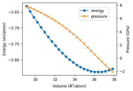
Finally, we plot the energy-volume curve along with the pressure-volume curve.

fig, ax = plt.subplots(figsize=(4.5, 3.5), dpi=90)

ax.plot(df.volume, df.energy, 'o-', label='energy')
ax2 = ax.twinx()
ax2.plot(df.volume, df.pressure, 'x-', color='C1', label='pressure')

ax.set_xlabel('Volume (Å$^3$/atom)')
ax.set_ylabel('Energy (eV/atom)')
ax2.set_ylabel('Pressure (GPa)')

fig.legend(loc='upper right', bbox_to_anchor=(0.85, 0.85));

Relaxation with a fixed cell

In some scenarios, it is helpful to keep the cell constant but still relax the atomic configuration. This can be done by setting the constant_cell keyword argument.

structure = bulk('PbTe', crystalstructure='rocksalt', a=6.6)
structure.cell *= 1.1 ** (1 / 3)  # we strain the cell like above
calc = CPUNEP('nep-PbTe.txt')
structure.calc = calc

We save the cell and atomic positions before relaxing.

positions_pre_relax = structure.get_positions()
cell_pre_relax = structure.get_cell()

The structure is then relaxed under the constraint that the cell is unchanged.

relax_structure(structure, constant_cell=True)

Finally, we make sure that the atoms moved but that the cell did not change.

# Make sure that the atoms moved
assert not np.allclose(positions_pre_relax, structure.get_positions())

# And make sure that the cell didn't change
assert np.allclose(cell_pre_relax, structure.get_cell())