Elastic properties

import numpy as np
from ase.build import bulk
from ase.calculators.emt import EMT
from ase.io import read
from ase.units import GPa, kg
from calorine.calculators import CPUNEP
from calorine.tools import get_elastic_stiffness_tensor, get_force_constants, relax_structure
from matplotlib import pyplot as plt
from pandas import DataFrame

This tutorial illustrates the calculation of the elastic stiffness tensor \(c_{ij}\) and its relation to the sound velocity. In the first part we use silver in its face-centered cubic (FCC) ground state structure described by an effective medium theory (EMT) potential as a particular simple example. In the second part we then consider the orthorhombic structure of CsPbI3, which allows us to demonstrate the difference between relaxed \(c_{ij}\) and clamped elastic constants \(c_{ij}^0\).

For background on crystal elasticity and the role of symmetry you can consult, e.g., Nye, Physical Properties of Crystals: Their Representation by Tensors and Matrices, Oxford University Press (1957).

All models and structures required for running this and the other tutorial notebooks can be obtained from Zenodo. The files are also available in the tutorials/ folder in the GitLab repository.

Face-centered cubic silver

Elastic constants and relation to sound velocities

First we set up the primitive structure of FCC Ag and relax the cell.

structure = bulk('Ag')
calculator = EMT()
structure.calc = calculator
relax_structure(structure, fmax=0.0001)

The elastic stiffness tensor \(c_{ij}\) can then be readily calculated using the get_elastic_stiffness_tensor function. The latter applies a series of deformations to the cell and fits the resulting strain energy to a Taylor expansion in strain, in which the components of the elastic stiffness tensor appear as expansion coefficients.

cij = get_elastic_stiffness_tensor(structure)
with np.printoptions(precision=1, suppress=True):
    print(cij)

[[125.9  87.3  87.3   0.   -0.    0. ]
 [ 87.3 125.9  87.3  -0.    0.    0. ]
 [ 87.3  87.3 125.9  -0.   -0.    0. ]
 [ -0.   -0.   -0.   54.2  -0.   -0. ]
 [ -0.    0.   -0.   -0.   54.2  -0. ]
 [  0.    0.    0.   -0.   -0.   54.2]]

The elastic constants are related to the sound velocity along different crystal directions. In particular \(c_{11}\) is related to the longitudinal speed of sound along \(\left<100\right>\) in the long-wavelength limit (i.e., \(\boldsymbol{q}\rightarrow 0\)) according to

\[c_s^{\left<100\right>} = \sqrt{\frac{c_{11}}{\rho}},\]

where \(\rho\) is the mass density of the material.

Let us now test this relationship. For simplicity of presentation, we use the conventional 4-atom unit cell in the following, for which the cell axes are oriented along the Cartesian directions.

structure = bulk('Ag', cubic=True)
calculator = EMT()
structure.calc = calculator
relax_structure(structure, fmax=0.0001)

We compute the force constants using the get_force_constants function and then use methods of the Phonopy object returned by the latter to calculate the group velocities at \(\boldsymbol{q}=(\delta, 0, 0)\) with \(\delta = 0.01\). This \(\boldsymbol{q}\)-point lies along \(\left<100\right>\) and the small \(\delta\)-value mimics the long-wavelength limit, i.e., \(\boldsymbol{q} \rightarrow 0\).

phonon = get_force_constants(structure, calculator, [2, 2, 2])
phonon.run_band_structure([[[0.01, 0, 0]]], with_group_velocities=True)
band = phonon.get_band_structure_dict()

Next we select the speed of sound of the LA branch and convert it to SI unitss (m/s).

group_velocities = np.linalg.norm(band['group_velocities'][0], axis=2) * 1e-10 / 1e-12  # Å/ps --> m/s
speed_of_sound = group_velocities[0][2]
print(f'speed of sound, LA, 100 : {speed_of_sound:7.1f} m/s')

speed of sound, LA, 100 :  3415.1 m/s

Combining the speed of sound with the mass density, then yields the elastic constant \(c_{11}\).

density = np.sum(structure.get_masses()) / structure.get_volume() / kg / 1e-30  # amu/Å^3 --> kg/m^3
print(f'density                 : {density:7.1f} kg/m^3')

elastic_constant = speed_of_sound ** 2 * density * 1e-9  # Pa --> GPa
print(f'elastic constant c11    : {elastic_constant:7.1f} GPa')

density                 : 10677.9 kg/m^3
elastic constant c11    :   124.5 GPa

The result of 124.5 GPa is in good agreement with the value of 125.9 GPa obtained above by direct evaluation of the elastic stiffness tensor.

Presssure dependence

We can now also readily evaluate the variation of the elastic constants with pressure.

data = []
for volsc in np.arange(0.88, 1.05, 0.04):
    structure_strained = structure.copy()
    cell = structure_strained.get_cell()
    cell *= volsc ** (1 / 3)
    structure_strained.set_cell(cell, scale_atoms=True)
    structure_strained.calc = calculator
    relax_structure(structure_strained, constant_volume=True)

    cij_rlx = get_elastic_stiffness_tensor(structure_strained)
    pressure = -np.sum(structure_strained.get_stress()[:3]) / 3 / GPa

    data.append(dict(volsc=volsc,
                     pressure=pressure,
                     volume=structure_strained.get_volume() / len(structure_strained),
                     c11=cij_rlx[0][0],
                     c12=cij_rlx[0][1],
                     c44=cij_rlx[3][3],
                    ))
df = DataFrame(data)

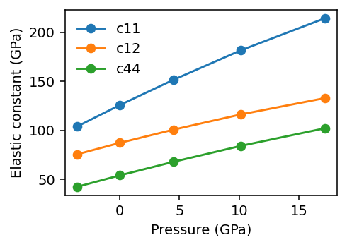
The results show a stiffening of the elastic constants with pressure, which is expected for this system.

fig, ax = plt.subplots(figsize=(3.6, 2.6), dpi=140)

for col in df:
    if not col.startswith('c'):
        continue
    ax.plot(df.pressure, df[col], 'o-', label=col)

ax.set_xlabel('Pressure (GPa)')
ax.set_ylabel('Elastic constant (GPa)')
ax.legend(frameon=False)

plt.tight_layout()

CsPbI3

In materials with internal degrees of freedom one can distinguish the so-called relaxed \(c_{ij}\) and clamped elastic constants \(c_{ij}^0\). In the former case, the ionic positions are allowed to relax after application of a macroscopic strain, whereas in the latter the relative coordinates are kept fixed.

To illustrate this effect, we here consider the elastic stiffness tensors in orthorhombic structure of CsPbI3, which we describe using a neuroevolution potential (NEP) taken from Fransson et al..

structure = read('CsPbI3-orthorhombic-Pnma.xyz')
calculator = CPUNEP('nep-CsPbI3-SCAN.txt')
structure.calc = calculator
relax_structure(structure, fmax=0.0001)

Next we can compute the relaxed (clamped=True; default) and clamped (clamped=False) elastic stiffness tensors. Since this is a rather soft material, we tighten the condition on the convergence of the forces (fmax=1e-5).

cij_rlx = get_elastic_stiffness_tensor(structure, fmax=1e-5)
cij_clamped = get_elastic_stiffness_tensor(structure, clamped=True)

with np.printoptions(precision=1, suppress=True):
    print('Relaxed elastic constants')
    print(cij_rlx)
    print('')
    print('Clamped elastic constants')
    print(cij_clamped)

Relaxed elastic constants
[[16.7 14.9 10.1 -0.  -0.   0. ]
 [14.9 25.3  9.5  0.  -0.   0. ]
 [10.1  9.5 31.1 -0.   0.  -0. ]
 [-0.   0.  -0.   6.1  0.  -0. ]
 [-0.  -0.   0.   0.   4.6 -0. ]
 [ 0.   0.  -0.  -0.  -0.  11.4]]

Clamped elastic constants
[[31.1 17.7  5.9  0.  -0.  -0. ]
 [17.7 34.9  5.2  0.  -0.   0. ]
 [ 5.9  5.2 46.8 -0.   0.  -0. ]
 [ 0.   0.  -0.   7.  -0.  -0. ]
 [-0.  -0.   0.  -0.   6.5  0. ]
 [-0.   0.  -0.  -0.   0.  18.4]]

Evidently in this material there is a pronounced difference between the relaxed and clamped elastic constants, which is related to the rather soft interactions.