Accessing NEP descriptors

This tutorial demonstrates the basic functionality available for the analysis of NEP models. Specifically, the interface exposes convenience functions for calculating per-atom descriptors, energies, forces, virials/stresses, dipoles and latent space representations for Atoms objects.

All models and structures required for running this and the other tutorial notebooks can be obtained from Zenodo. The files are also available in the tutorials/ folder in the GitLab repository.

We start by creating an Atoms object, which will serve as our prototype system for the extent of this tutorial, and by importing the get_descriptors, get_potential_forces_and_virials, get_dipole and get_latent_space functions from the calorine.nep submodule.

from ase.io import read
from ase.build import bulk
import matplotlib.pyplot as plt
from calorine.nep import get_descriptors, \
                         get_potential_forces_and_virials, \
                         get_dipole, \
                         get_latent_space

structure = bulk('PbTe', crystalstructure='rocksalt', a=6.7)

We can now compute the descriptors, energies, forces and virials for our system by calling get_descriptors and get_potential_forces_and_virials. To this end, we pass the atomic structure together with the path to a NEP model file. Here, we use a NEP4 model for PbTe.

descriptors = get_descriptors(structure, model_filename='nep-PbTe.txt')

per_atom_energies, forces, virials = \
    get_potential_forces_and_virials(structure, model_filename='nep-PbTe.txt')

print(f'Shape of descriptors: {descriptors.shape}')
print(f'Energy (eV):\n {per_atom_energies}')
print(f'Forces (eV/Å):\n {forces}')
print(f'Virials (eV):\n {virials}')

Shape of descriptors: (2, 30)
Energy (eV):
 [-1.94265756 -5.72050595]
Forces (eV/Å):
 [[ 9.43689571e-16 -2.08961602e-16 -4.73106562e-16]
 [-9.50628465e-16  2.08961602e-16  4.73106562e-16]]
Virials (eV):
 [[-9.29170315e-01 -1.43931046e-16 -3.65311983e-17 -1.56074110e-16
  -9.29170315e-01  5.89805982e-17 -3.65311983e-17  5.72458747e-17
  -9.29170315e-01]
 [ 1.08945431e-01 -5.20081776e-16 -1.04008905e-16 -5.20081776e-16
   1.08945431e-01  1.31913488e-16 -1.21356140e-16  1.24974594e-16
   1.08945431e-01]]

get_descriptors can also be called without supplying a NEP model file, in which case a dummy NEP2 model will be generated on-the-fly. The dummy model has all parameter values set to 1. Note that this model does not differentiate different atom species. Thus, supplying your own trained NEP model file is recommended for most applications.

descriptors = get_descriptors(structure)
print(f'Shape of descriptors: {descriptors.shape}')

Shape of descriptors: (2, 52)

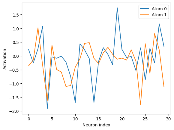
Accessing latent space representations

The latent space representation of a structure can be obtained using the function get_latent_space. The latent space is a matrix, with shape (number_of_atoms, number_of_neurons) where number_of_neurons is the number of neurons in the hidden layer in the neural network.

%matplotlib inline
structure = bulk('PbTe', crystalstructure='rocksalt', a=6.7)
latent = get_latent_space(structure, model_filename='nep-PbTe.txt')

print(f'Shape of latent space: {latent.shape}')

fig, ax = plt.subplots()
ax.plot(latent[0,:], label='Atom 0')
ax.plot(latent[1,:], label='Atom 1')
ax.set_xlabel('Neuron index')
ax.set_ylabel('Activation')
ax.legend(loc='best');

Shape of latent space: (2, 30)