Using the ASE calculators

This tutorial demonstrates how to use the ASE calculators for neuroevolution potentials (NEP), which allow one to calculate energies, forces and stresses for an atomic configuration, specified in the form of an Atoms object. This enables one to programmatically calculate properties that would otherwise require writing a large number of GPUMD input files and potentially tedious extraction of the results.

calorine provides two different ASE calculators for NEP calculations, one that uses the GPU implementation and one that uses the CPU implementation of NEP. For smaller calculations the CPU calculators is usually more performant. For very large simulations and for comparison the GPU calculator can be useful as well.

All models and structures required for running this and the other tutorial notebooks can be obtained from Zenodo. The files are also available in the tutorials/ folder in the GitLab repository.

CPU-based calculator

Basic usage

First we define an atomic structure in the form of an Atoms object. Next we create a calculator instance by specifying the path to a NEP model file in nep.txt format. In this tutorial, we use a NEP4 model for PbTe. This model is included in the calorine/tutorials/ folder. Finally, we attach the calculator to the Atoms object.

from ase.io import read
from ase.build import bulk
from calorine.calculators import CPUNEP

structure = bulk('PbTe', crystalstructure='rocksalt', a=6.7)
calc = CPUNEP('nep-PbTe.txt')
structure.calc = calc

Now, we can readily calculate energies, forces and stresses.

print('Energy (eV):', structure.get_potential_energy())
print('Forces (eV/Å):\n', structure.get_forces())
print('Stress (GPa):\n', structure.get_stress())

Energy (eV): -7.663163505693399
Forces (eV/Å):
 [[ 9.43689571e-16 -2.08961602e-16 -4.73106562e-16]
 [-9.50628465e-16  2.08961602e-16  4.73106562e-16]]
Stress (GPa):
 [ 1.09085876e-02  1.09085876e-02  1.09085876e-02 -2.53879747e-18
  1.86911426e-18  8.83104401e-18]

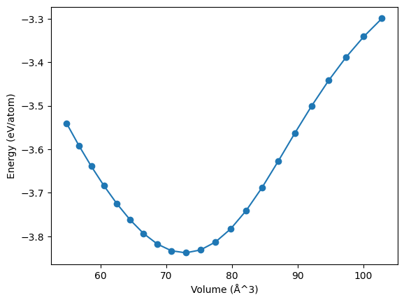
Calculate energy-volume curve

To demonstrate the capabilities of the ASE calculator, we will now calculate an energy-volume curve with the PbTe potential.

%matplotlib inline
import numpy as np
import matplotlib.pyplot as plt

energies = []
volumes = []

structure_copy = structure.copy()
original_cell = structure.cell.copy()

structure_copy.calc = calc

for scale in np.arange(0.9, 1.11, 0.01):
    structure_copy.set_cell(scale * original_cell, scale_atoms=True)
    volumes.append(structure_copy.get_volume())
    energies.append(structure_copy.get_potential_energy() / len(structure_copy))

fig, ax = plt.subplots()
ax.plot(volumes, energies, '-o')
ax.set_xlabel('Volume (Å^3)')
ax.set_ylabel('Energy (eV/atom)');

Calculate dipole moments

The calculator also supports the calculation of dipole moments. Note that you must have a NEP model trained to predict dipoles; otherwise the output will be nonsensical. Refer to the GPUMD documentation for information on how to train a dipole model.

The model and structure are included in the calorine/tutorials/ folder.

dipole_model = 'nep-PTAF-dipole.txt'
structure = read('PTAF-monomer.xyz')
calc = CPUNEP(dipole_model)
structure.calc = calc

dipole = structure.get_dipole_moment()
dft_dipole = structure.info['dipole']

print('DFT dipole moment:'.ljust(30) +  f'{dft_dipole} a.u.')
print(f'NEP predicted dipole moment:'.ljust(30) + f'{dipole} a.u.')

DFT dipole moment:            [4.85503 0.07166 0.16004] a.u.
NEP predicted dipole moment:  [4.78034782 0.03274603 0.04843106] a.u.

GPU-based calculator

The basic usage of the GPUNEP calculator class is completely analoguous to the CPUNEP calculator. We create an atomic structure and attach the calculator object.

from calorine.calculators import GPUNEP

structure = bulk('PbTe', crystalstructure='rocksalt', a=6.7)
calc = GPUNEP('nep-PbTe.txt')
structure.calc = calc

Afterwards we can readily obtain energies, forces, and stresses.

print('Energy (eV):', structure.get_potential_energy())
print('Forces (eV/Å):\n', structure.get_forces())
print('Stresses (eV/Å^3):\n', structure.get_stress())

Energy (eV): -7.6631630659
Forces (eV/Å):
 [[ 2.91459e-07  2.77747e-07  1.82196e-07]
 [-2.91459e-07 -2.77747e-07 -1.82196e-07]]
Stresses (eV/Å^3):
 [ 1.09085639e-02  1.09085643e-02  1.09085477e-02 -3.55200559e-10
 -3.55200534e-10  9.51932078e-10]

Temporary and specified directories

Under the hood, the GPUNEP calculator creates a directory and writes the input files necessary to run GPUMD. By default, this is done in temporary directories that are automatically removed once the calculations has finished. It is also possible to run in a user-specified directory that will be kept after the calculations finish. This is especially useful when running molecular dynamics simulations (see below).

calc.set_directory('my_directory')
structure.get_potential_energy()

-7.6631630659

After this is run, there should be a new directory, my_directory, in which input and output files from GPUMD are available. This can be useful for debugging.

Running custom molecular dynamics simulations

To take advantage of the Python workflow as well as raw speed of the GPU accelerated NEP implementation, the GPUNEP calculator contains a convenience function for running customized molecular dynamics simulations. This should typically be done in a specified directory. The parameters of the run.in file are specified as a list of tuples with two elements, the first being the keyword name and the second any arguments to that keyword.

calc.set_directory('my_md_simulation')
supercell = structure.repeat(5)
structure.calc = calc
parameters = [('velocity', 300),
              ('dump_thermo', 100),
              ('dump_position', 100),
              ('ensemble', ('nvt_lan', 300, 300, 100)),
              ('run', 1000)]
calc.run_custom_md(parameters)

Once this is run, the results are available in the folder my_md_simulations.