Structure generation and NEP training

This tutorial demonstrates a simple approach for generating an initial set of training structures for the construction of a NEP for bulk aluminium.

Structure generation

First, we identify all the relevant prototype structures (FCC, BCC, HCP, diamond) that we want to include in the training set.

Next, we generate strained and deformed versions of the prototype structures. Additionally, we include rattled supercells (of various sizes) with random atomic displacements.

Lastly, we note that if one wants to consider mixed alloy systems, defects, surfaces etc, one needs to be more careful during structure generation to include training structures such that one spans that part of the configurational space.

Training

We use the function setup_training in calorine in order to set up and prepare all relevant files for the training. Here, we use the ASE EMT calculator (instead of density functional theory) to compute energies, forces and stresses for the training structures to make the tutorial more lightweight. After the NEP is trained we carry out some simple analysis of the model, specifically by constructing parity plots.

Note that the approach in this tutorial can be used to construct an initial NEP for the given system. However, after training this initial model it is recommened to carry out a few iterations of active learning based on, e.g., molecular dynamics simulations to enhance the training set.

import numpy as np
from ase.build import bulk, make_supercell, surface
from ase.calculators.emt import EMT
from ase.io import write
from calorine.tools import relax_structure
from hiphive.structure_generation import generate_mc_rattled_structures

Prototype structures

First, we collect all prototype structures of interest.

prototype_structures = {}
prototype_structures['fcc'] = bulk('Al', crystalstructure='fcc', a=4.05, cubic=True)
prototype_structures['bcc'] = bulk('Al', crystalstructure='bcc', a=3.12, cubic=True)
prototype_structures['hcp'] = bulk('Al', crystalstructure='hcp', a=2.82, c=4.47)
prototype_structures['diamond'] = bulk('Al', crystalstructure='diamond', a=6.1, cubic=True)

Generation of strained and deformed prototype structures

Next, we generate strained and deformed versions of prototype structures. strain_lim sets the range on how much we can strain or deform the cell of prototype structures.

def generate_strained_structure(prim, strain_lim):
    strains = np.random.uniform(*strain_lim, (3, ))
    atoms = prim.copy()
    cell_new = prim.cell[:] * (1 + strains)
    atoms.set_cell(cell_new, scale_atoms=True)
    return atoms


def generate_deformed_structure(prim, strain_lim):
    R = np.random.uniform(*strain_lim, (3, 3))
    M = np.eye(3) + R
    atoms = prim.copy()
    cell_new = M @ atoms.cell[:]
    atoms.set_cell(cell_new, scale_atoms=True)
    return atoms


# parameters
strain_lim = [-0.05, 0.05]
n_structures = 15

training_structures = []
for name, prim in prototype_structures.items():
    for it in range(n_structures):
        prim_strained = generate_strained_structure(prim, strain_lim)
        prim_deformed = generate_deformed_structure(prim, strain_lim)

        training_structures.append(prim_strained)
        training_structures.append(prim_deformed)

print('Number of training structures:', len(training_structures))

Number of training structures: 120

Generation of rattled structures

We also include some rattled structures in the training set. One can use the functions generate_rattled_structures (for small displacements) and generate_mc_rattled_structures for larger displacements from hiphive, see the hiphive documentation for more details.

The d_min parameter approximatley corresponds to the smallest interatomic distance we would like to see in the MC-rattled structures, here set to about 90% of the nearest neighbor distance.

The rattle_std and n_iter determines how large the displacements will, the displacements generated will roughly be n_iter**0.5 * rattle_std.

Note that it can be useful to include supercells of various system sizes as done below.

n_structures = 5
rattle_std = 0.04
d_min = 2.3
n_iter = 20

size_vals = {}
size_vals['fcc'] = [(2, 2, 2), (3, 3, 3), (4, 4, 4)]
size_vals['bcc'] = [(2, 2, 2), (3, 3, 3), (4, 4, 4)]
size_vals['hcp'] = [(2, 2, 2), (3, 3, 3), (4, 4, 4)]
size_vals['diamond'] = [(2, 2, 2), (3, 3, 3)]

for name, prim in prototype_structures.items():
    for size in size_vals[name]:
        for it in range(n_structures):
            supercell = generate_strained_structure(prim.repeat(size), strain_lim)
            rattled_supercells = generate_mc_rattled_structures(supercell, n_structures=1, rattle_std=rattle_std, d_min=d_min, n_iter=n_iter)
            print(f'{name}, size {size}, natoms {len(supercell)},  volume {supercell.get_volume() / len(supercell):.3f}')
            training_structures.extend(rattled_supercells)

fcc, size (2, 2, 2), natoms 32,  volume 17.545
fcc, size (2, 2, 2), natoms 32,  volume 16.576
fcc, size (2, 2, 2), natoms 32,  volume 17.164
fcc, size (2, 2, 2), natoms 32,  volume 15.687
fcc, size (2, 2, 2), natoms 32,  volume 16.386
fcc, size (3, 3, 3), natoms 108,  volume 17.944
fcc, size (3, 3, 3), natoms 108,  volume 17.985
fcc, size (3, 3, 3), natoms 108,  volume 16.193
fcc, size (3, 3, 3), natoms 108,  volume 16.336
fcc, size (3, 3, 3), natoms 108,  volume 16.648
fcc, size (4, 4, 4), natoms 256,  volume 16.636
fcc, size (4, 4, 4), natoms 256,  volume 18.020
fcc, size (4, 4, 4), natoms 256,  volume 17.754
fcc, size (4, 4, 4), natoms 256,  volume 16.065
fcc, size (4, 4, 4), natoms 256,  volume 15.419
bcc, size (2, 2, 2), natoms 16,  volume 14.782
bcc, size (2, 2, 2), natoms 16,  volume 14.768
bcc, size (2, 2, 2), natoms 16,  volume 15.874
bcc, size (2, 2, 2), natoms 16,  volume 15.626
bcc, size (2, 2, 2), natoms 16,  volume 13.882
bcc, size (3, 3, 3), natoms 54,  volume 15.271
bcc, size (3, 3, 3), natoms 54,  volume 13.676
bcc, size (3, 3, 3), natoms 54,  volume 16.556
bcc, size (3, 3, 3), natoms 54,  volume 14.940
bcc, size (3, 3, 3), natoms 54,  volume 15.441
bcc, size (4, 4, 4), natoms 128,  volume 16.244
bcc, size (4, 4, 4), natoms 128,  volume 14.433
bcc, size (4, 4, 4), natoms 128,  volume 16.276
bcc, size (4, 4, 4), natoms 128,  volume 15.721
bcc, size (4, 4, 4), natoms 128,  volume 14.219
hcp, size (2, 2, 2), natoms 16,  volume 16.084
hcp, size (2, 2, 2), natoms 16,  volume 16.415
hcp, size (2, 2, 2), natoms 16,  volume 15.554
hcp, size (2, 2, 2), natoms 16,  volume 15.406
hcp, size (2, 2, 2), natoms 16,  volume 16.846
hcp, size (3, 3, 3), natoms 54,  volume 15.968
hcp, size (3, 3, 3), natoms 54,  volume 17.227
hcp, size (3, 3, 3), natoms 54,  volume 16.343
hcp, size (3, 3, 3), natoms 54,  volume 15.922
hcp, size (3, 3, 3), natoms 54,  volume 15.945
hcp, size (4, 4, 4), natoms 128,  volume 16.196
hcp, size (4, 4, 4), natoms 128,  volume 15.069
hcp, size (4, 4, 4), natoms 128,  volume 14.559
hcp, size (4, 4, 4), natoms 128,  volume 14.829
hcp, size (4, 4, 4), natoms 128,  volume 15.930
diamond, size (2, 2, 2), natoms 64,  volume 27.739
diamond, size (2, 2, 2), natoms 64,  volume 30.554
diamond, size (2, 2, 2), natoms 64,  volume 26.404
diamond, size (2, 2, 2), natoms 64,  volume 31.200
diamond, size (2, 2, 2), natoms 64,  volume 26.451
diamond, size (3, 3, 3), natoms 216,  volume 28.871
diamond, size (3, 3, 3), natoms 216,  volume 31.406
diamond, size (3, 3, 3), natoms 216,  volume 29.147
diamond, size (3, 3, 3), natoms 216,  volume 25.816
diamond, size (3, 3, 3), natoms 216,  volume 30.266

We can visualize and inspect the training structures using the view function in ASE.

from ase.visualize import view

print('Number of training structures:', len(training_structures))

view(training_structures)

Number of training structures: 175

<subprocess.Popen at 0x7f9cac51bbe0>

Training

We use the EMT calculator to compute the reference energies, forces and stresses. We change some of the default NEP hyper-parameters, such as the number of neurons to 30.

Note that we only train for 100,000 generations. In practice one should train until the model has converged, which typically requires many more generations.

# do reference calculations
for atoms in training_structures:
    atoms.calc = EMT()
    atoms.get_potential_energy()

from calorine.nep import setup_training

# prepare input for NEP construction
parameters = dict(version=4,
                  type=[1, 'Al'],
                  cutoff=[8, 4],
                  neuron=30,
                  generation=100000,
                  batch=1000000)

setup_training(parameters, training_structures, rootdir='model', overwrite=True, n_splits=10)

The cell above sets up all required files for training in the model/ directory. In model/nepmodel_full all structures are used for training, and in the model/nepmodel_split directories 90% of the structures are used for training and 10% for testing, which is known as K-fold cross validation with K=10.

Next, one needs to go into each model directory (model/nepmodel_full and model/nepmodel_split*) and run nep in order to start the training. The training is computationally expensive and here with about 200 training structures takes about 2 hours on a A100 GPU.

Analysis of the model

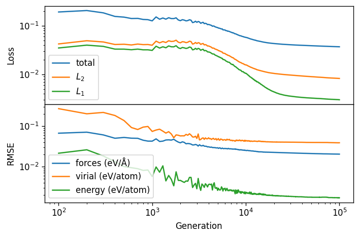
First we plot the total loss function, the L1 and L2 regularization part of the loss function and the corresponding RMSE (root mean squared error) for the full training set of the nepmodel_full model.

We can see that the training has more or less converged with 100,000 generations.

import pandas as pd
from ase.units import GPa
from calorine.nep import get_parity_data, read_loss, read_structures
from matplotlib import pyplot as plt
from pandas import DataFrame, concat as pd_concat
from sklearn.metrics import r2_score, mean_squared_error

loss = read_loss('model/nepmodel_full/loss.out')

fig, axes = plt.subplots(figsize=(6.0, 4.0), nrows=2,sharex=True, dpi=120)

ax = axes[0]
ax.set_ylabel('Loss')
ax.plot(loss.total_loss, label='total')
ax.plot(loss.L2, label='$L_2$')
ax.plot(loss.L1, label='$L_1$')
ax.set_yscale('log')
ax.legend()

ax = axes[1]
ax.plot(loss.RMSE_F_train, label='forces (eV/Å)')
ax.plot(loss.RMSE_V_train, label='virial (eV/atom)')
ax.plot(loss.RMSE_E_train, label='energy (eV/atom)')
ax.set_xscale('log')
ax.set_yscale('log')
ax.set_xlabel('Generation')
ax.set_ylabel('RMSE')
ax.legend()

plt.tight_layout()
fig.subplots_adjust(hspace=0, wspace=0)
fig.align_ylabels(axes)

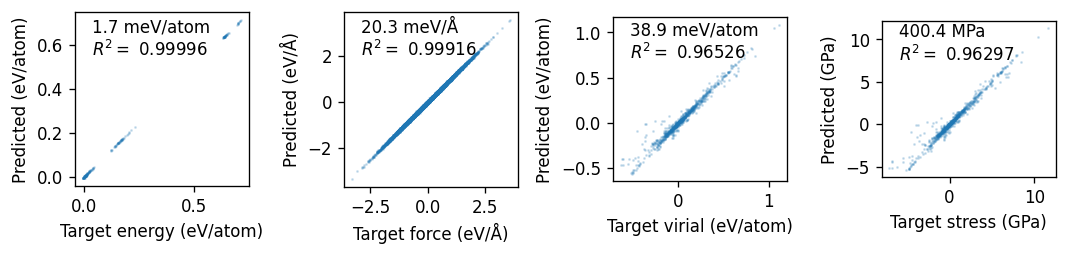
Finally, we plot the parity plots using the read_structures and get_parity_data functions. We can see that the model does a good job of reproducing the reference data.

training_structures, _ = read_structures('model/nepmodel_full')

units = dict(
    energy='eV/atom',
    force='eV/Å',
    virial='eV/atom',
    stress='GPa',
)

fig, axes = plt.subplots(figsize=(9.0, 2.6), ncols=4, dpi=120)
kwargs = dict(alpha=0.2, s=0.5)

for icol, (prop, unit) in enumerate(units.items()):
    df = get_parity_data(training_structures, prop, flatten=True)
    R2 = r2_score(df.target, df.predicted)
    rmse = mean_squared_error(df.target, df.predicted, squared=False)

    ax = axes[icol]
    ax.set_xlabel(f'Target {prop} ({unit})')
    ax.set_ylabel(f'Predicted ({unit})')
    ax.scatter(df.target, df.predicted, **kwargs)
    ax.set_aspect('equal')
    mod_unit = unit.replace('eV', 'meV').replace('GPa', 'MPa')
    ax.text(0.1, 0.75, f'{1e3*rmse:.1f} {mod_unit}\n' + '$R^2= $' + f' {R2:.5f}', transform=ax.transAxes)

fig.tight_layout()