Training a tensorial NEP#
This tutorial demonstrates how to train a tensorial neuroevolution potential (TNEP), as presented in Xu et al. (2024). We will train a model for predicting the molecular dipole in water using the data published alongside the paper, use the model to run molecular dynamics, and from the trajectory extract and predict the IR spectrum of water.
In short, TNEP extends the NEP formalism which predicts the (non-physical) per-atom energies \(U_i\) as a function of atom-centered descriptors \(q_i^\gamma\),
We can calculate the gradients of \(U_i\) to analytically obtain the partial force \(\partial U_i / \partial r_{ij}^\nu\), where \(r_{ij}^\nu\) is the \(\nu\)-component of the interatomic distance vector \(\boldsymbol{r}_{ij} = \boldsymbol{r}_j - \boldsymbol{r}_i\). The basis for predicting tensorial properties within the TNEP framework is the partial force and the rank-2 virial tensor \(W^{\mu \nu}\), denoted as
Rank-1 tensors such as the molecular dipole \(\boldsymbol{\mu}\) might naïvely be predicted based on the partial force directly. However, this does not work as the partial forces sum to zero per construction. To circumvent this problem, the TNEP framework draws inspiration from the atomic virial, and defines rank-1 tensors based on a contraction of the rank-2 virial tensor with a vector,
For rank-2 tensors such as molecular polarization \(\boldsymbol{\alpha}\) or electric susecptibility \(\boldsymbol{\chi}\), the virial tensor is slightly adapted for numerical stability,
\(\delta^{\mu \nu}\) is the Kronecker delta, and helps stabilize the prediction of rank-2 tensor as the diagonal elements often are large than the off-diagonal elements.
Loading the dataset#
We can obtain DFT training data of structures with the molecular dipole for water from Zenodo, where we will obtain the file dipole_bulk_water.zip. The file is roughly 1.6MB in size.
[1]:
!wget -P tnep-tutorial/ https://zenodo.org/records/10257363/files/dipole_bulk_water.zip
--2026-02-13 15:20:41--  https://zenodo.org/records/10257363/files/dipole_bulk_water.zip
Resolving zenodo.org (zenodo.org)... 188.185.43.153, 188.185.48.75, 188.184.98.114, ...
Connecting to zenodo.org (zenodo.org)|188.185.43.153|:443... connected.
HTTP request sent, awaiting response... 200 OK
Length: 1550097 (1.5M) [application/octet-stream]
Saving to: ‘tnep-tutorial/dipole_bulk_water.zip’

dipole_bulk_water.z 100%[===================>]   1.48M  5.36MB/s    in 0.3s

2026-02-13 15:20:41 (5.36 MB/s) - ‘tnep-tutorial/dipole_bulk_water.zip’ saved [1550097/1550097]
[2]:
!unzip tnep-tutorial/dipole_bulk_water.zip -d tnep-tutorial/
Archive:  tnep-tutorial/dipole_bulk_water.zip
  inflating: tnep-tutorial/dipole_bulk_water/nep.in
  inflating: tnep-tutorial/dipole_bulk_water/nep.txt
  inflating: tnep-tutorial/dipole_bulk_water/test.xyz
  inflating: tnep-tutorial/dipole_bulk_water/train.xyz
We load the training and test structures using ASE.
[3]:
from ase.io import read

train_structures = read('tnep-tutorial/dipole_bulk_water/train.xyz', ':')
test_structures = read('tnep-tutorial/dipole_bulk_water/test.xyz', ':')

print(f'{len(train_structures)} structures in the training set, and {len(test_structures)} structures in the test set.')
500 structures in the training set, and 500 structures in the test set.
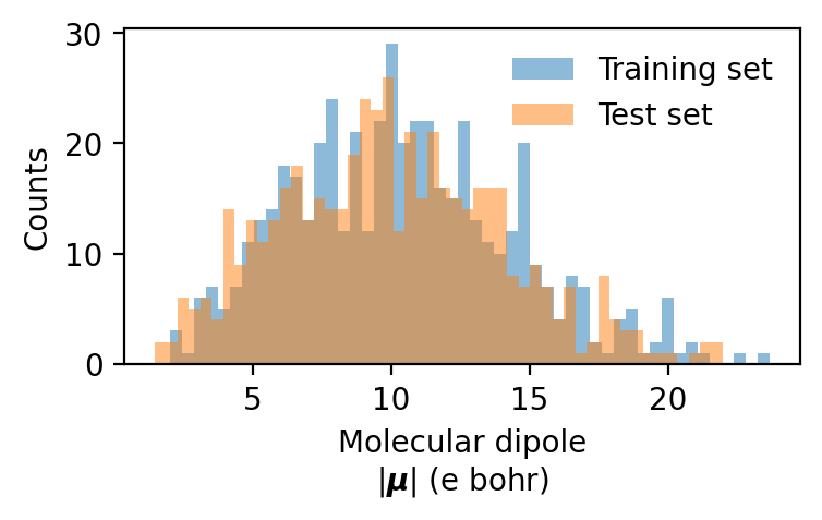
We can also inspect the molecular dipoles:
[4]:
import numpy as np
import matplotlib.pyplot as plt

train_dipole_magnitudes = np.linalg.norm([structure.get_dipole_moment() for structure in train_structures], axis=1)
test_dipole_magnitudes = np.linalg.norm([structure.get_dipole_moment() for structure in test_structures], axis=1)
[5]:
fig, ax = plt.subplots(figsize=(4, 2), dpi=200)
nbins = 50
ax.hist(train_dipole_magnitudes, bins=nbins, label='Training set', alpha=0.5)
ax.hist(test_dipole_magnitudes, bins=nbins, label='Test set', alpha=0.5)
ax.set(xlabel='Molecular dipole\n' + r'$|\boldsymbol{\mu}|$ (e bohr)', ylabel='Counts')
ax.legend(loc='upper right', frameon=False)
[5]:
<matplotlib.legend.Legend at 0x7ae25be48e30>
Preparing training#
We can now use setup_training from calorine to prepare training of the model.
Please refer to the GPUMD documentation for details on the different parameters set below. The most important of these is model_type=1, which signals to the nep executable that we aim to train a rank-1 tensorial model.
[6]:
from calorine.nep import setup_training

# prepare input for NEP construction
parameters = dict(version=4,
                  type=[2, 'O', 'H'],
                  model_type=1,
                  cutoff=[6, 4],
                  n_max=[6, 6],
                  basis_size=[10, 10],
                  l_max=[4, 2, 1],
                  neuron=10,
                  population=80,
                  lambda_1=0.0005,
                  lambda_2=0.0005,
                  generation=50000,
                  save_potential=[5000, 0, 1],
                  batch=500)

setup_training(parameters, train_structures, rootdir='tnep-tutorial', overwrite=True, mode='bagging', train_fraction=1)
/home/elindgren/repos/calorine/calorine/nep/io.py:94: UserWarning: Failed to retrieve stresses for structure
  warn('Failed to retrieve stresses for structure')
The cell above sets up all required files for training in the tnep-tutorial/nepmodel_full directory. Next, one needs to go to tnep-tutorial/nepmodel_full and run nep in order to start the training. The training is computationally expensive and here with 500 training structures takes about 5 hours on an A100 GPU.
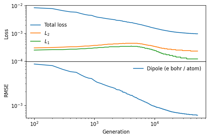
Analysis of the model#
We can now analyze the training of the model trained on all available data, nepmodel_full.
[7]:
from calorine.nep import get_parity_data, read_loss, read_structures

loss = read_loss('tnep-tutorial/nepmodel_full/loss.out')

fig, axes = plt.subplots(figsize=(6.0, 4.0), nrows=2,sharex=True, dpi=120)

ax = axes[0]
ax.set_ylabel('Loss')
ax.plot(loss.total_loss, label='Total loss')
ax.plot(loss.L2, label='$L_2$')
ax.plot(loss.L1, label='$L_1$')
ax.set_yscale('log')
ax.legend(frameon=False)

ax = axes[1]
ax.plot(loss.RMSE_P_train, label='Dipole (e bohr / atom)')
ax.set_xscale('log')
ax.set_yscale('log')
ax.set_xlabel('Generation')
ax.set_ylabel('RMSE')
ax.legend(frameon=False)

fig.tight_layout()
fig.subplots_adjust(hspace=0, wspace=0)
fig.align_ylabels(axes)
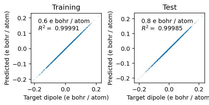
From the parity plots below, we see that the model is able to accurately reproduce the reference data.
[8]:
from pandas import DataFrame
from calorine.nep import read_structures, get_parity_data
from calorine.calculators import CPUNEP

training_structures, _ = read_structures('./tnep-tutorial/nepmodel_full')
train_df = get_parity_data(training_structures, 'dipole', flatten=True)

# Evaluate the model on the test set to get predictions
test_structures = read('tnep-tutorial/dipole_bulk_water/test.xyz', ':')
test_dipole_targets = np.array([structure.get_dipole_moment()/len(structure) for structure in test_structures]).flatten()
test_dipole_predictions =  np.array([CPUNEP('./tnep-tutorial/nepmodel_full/nep.txt', structure).get_dipole_moment()/len(structure)
                                     for structure in test_structures]).flatten()

test_df = DataFrame(np.vstack([test_dipole_predictions, test_dipole_targets]).T, columns=['predicted', 'target'])
[9]:
from sklearn.metrics import r2_score, mean_squared_error
unit = 'e bohr / atom'

fig, axes = plt.subplots(figsize=(5, 2.5), ncols=2, dpi=140)
kwargs = dict(alpha=0.2, s=0.5)

for icol, (df, label) in enumerate(zip([train_df, test_df], ['Training', 'Test'])):
    R2 = r2_score(df.target, df.predicted)
    rmse = np.sqrt(mean_squared_error(df.target, df.predicted))

    ax = axes[icol]
    ax.set_xlabel(f'Target dipole ({unit})')
    ax.set_ylabel(f'Predicted ({unit})')
    ax.set_title(label)
    ax.scatter(df.target, df.predicted, **kwargs)
    ax.set_aspect('equal')
    mod_unit = unit.replace('eV', 'meV').replace('GPa', 'MPa')
    ax.text(0.1, 0.75, f'{1e3*rmse:.1f} {mod_unit}\n' + '$R^2= $' + f' {R2:.5f}', transform=ax.transAxes)

fig.tight_layout()
Predicting the IR spectrum of water#
Equipped with an ensemble of trained TNEP models, we can now run a molecular dynamics simulation and predict the IR spectrum.
We will compute the IR spectrum from the Fourier transform of the autocorrelation function of the dipole. In the classical approximation and assuming an isotropic sample, the IR absorption cross section \(\sigma(\omega)\) can be obtained as
Refer to the paper by Xu et al. (2024) for details.
In order to resolve all atomic vibrations and avoid aliasing we thus need to write the dipoles sufficiently often. Given that that the O-H stretch mode has a frequency of around 3600 cm\(^{-1}\), corresponding to a period time of about 9.5 fs, we write the dipoles approximately every 2 fs to avoid aliasing and collect decent statistics.
We additionally need a regular NEP model for the potential energy surface (PES). We can also obtain this from the Zenodo record from Xu et al.
[10]:
!wget -P tnep-tutorial/ https://zenodo.org/records/10257363/files/nep_PES_water.txt
--2026-02-13 15:20:46--  https://zenodo.org/records/10257363/files/nep_PES_water.txt
Resolving zenodo.org (zenodo.org)... 188.184.103.118, 188.185.43.153, 137.138.153.219, ...
Connecting to zenodo.org (zenodo.org)|188.184.103.118|:443... connected.
HTTP request sent, awaiting response... 200 OK
Length: 177789 (174K) [text/plain]
Saving to: ‘tnep-tutorial/nep_PES_water.txt’

nep_PES_water.txt   100%[===================>] 173.62K  --.-KB/s    in 0.1s

2026-02-13 15:20:47 (1.15 MB/s) - ‘tnep-tutorial/nep_PES_water.txt’ saved [177789/177789]
We set up the molecular dynamics simulation using the GPUNEP calculator from calorine. We first run a 100 ps simulation in the NPT ensemble to thermalize the system, and then run a 50 ps simulation in the NVT ensemble where we write the dipoles every 2 fs (4 timesteps).
[11]:
%%time
from calorine.calculators import GPUNEP

potential_model = './tnep-tutorial/nep_PES_water.txt'

run_parameters = [
    ('potential', '../nep_PES_water.txt'),
    ('potential', '../nepmodel_full/nep.txt'),  # TNEP model
    ('time_step', 0.5),
    ('velocity', '300'),
    ('ensemble', ('npt_ber', 300, 300, 100, 0, 2, 100)),
    ('dump_thermo', 100),
    ('run', 20000),
    ('ensemble', ('nvt_lan', 300, 300, 100)),
    ('dump_thermo', 100),
    ('dump_dipole', 4),
    ('dump_position', 4),
    ('run', 20000),
]

# We start from the first frame of the training set
structure = train_structures[0]
structure.wrap()

calc = GPUNEP(potential_model, directory='./tnep-tutorial/md', command='gpumd 2>&1')
structure.calc = calc
calc.run_custom_md(run_parameters)
***************************************************************
*                 Welcome to use GPUMD                        *
*     (Graphics Processing Units Molecular Dynamics)          *
*                     version 4.8                             *
*              This is the gpumd executable                   *
***************************************************************


---------------------------------------------------------------
Compiling options:
---------------------------------------------------------------

DEBUG is off: Use different PRNG seeds for different runs.

---------------------------------------------------------------
GPU information:
---------------------------------------------------------------

number of GPUs = 1
Device id:                   0
    Device name:             NVIDIA GeForce RTX 3080 Ti
    Compute capability:      8.6
    Amount of global memory: 11.6227 GB
    Number of SMs:           80

---------------------------------------------------------------
Started running GPUMD.
---------------------------------------------------------------


---------------------------------------------------------------
Started initializing positions and related parameters.
---------------------------------------------------------------

Number of atoms is 96.
Use periodic boundary conditions along x.
Use periodic boundary conditions along y.
Use periodic boundary conditions along z.
Box matrix h = [a, b, c] is
    9.9399900000e+00    0.0000000000e+00    0.0000000000e+00
    0.0000000000e+00    9.9399900000e+00    0.0000000000e+00
    0.0000000000e+00    0.0000000000e+00    9.9399900000e+00
Inverse box matrix g = inv(h) is
    1.0060372294e-01    0.0000000000e+00    0.0000000000e+00
    0.0000000000e+00    1.0060372294e-01    0.0000000000e+00
    0.0000000000e+00    0.0000000000e+00    1.0060372294e-01
Do not specify initial velocities here.
Have no grouping method.
There are 2 atom types.
    32 atoms of type 0.
    64 atoms of type 1.
Initialized velocities with default T = 300 K.

---------------------------------------------------------------
Finished initializing positions and related parameters.
---------------------------------------------------------------


---------------------------------------------------------------
Started executing the commands in run.in.
---------------------------------------------------------------

Use the NEP4 potential with 2 atom types.
    type 0 (O with Z = 8).
    type 1 (H with Z = 1).
    radial cutoff = 6 A.
    angular cutoff = 4 A.
    MN_radial = 251.
    enlarged MN_radial = 314.
    enlarged MN_angular = 100.
    n_max_radial = 9.
    n_max_angular = 7.
    basis_size_radial = 9.
    basis_size_angular = 7.
    l_max_3body = 4.
    l_max_4body = 2.
    l_max_5body = 0.
    ANN = 50-100-1.
    number of neural network parameters = 10401.
    number of descriptor parameters = 656.
    total number of parameters = 11057.
Use the NEP4 potential with 2 atom types.
    type 0 (O with Z = 8).
    type 1 (H with Z = 1).
    radial cutoff = 6 A.
    angular cutoff = 4 A.
    MN_radial = 112.
    enlarged MN_radial = 140.
    enlarged MN_angular = 49.
    n_max_radial = 6.
    n_max_angular = 6.
    basis_size_radial = 10.
    basis_size_angular = 10.
    l_max_3body = 4.
    l_max_4body = 2.
    l_max_5body = 1.
    ANN = 49-10-1.
    number of neural network parameters = 1021.
    number of descriptor parameters = 616.
    total number of parameters = 1637.
Time step for this run is 0.5 fs.
Initialized velocities with input T = 300 K.
Use NPT ensemble for this run.
    choose the Berendsen method.
    initial temperature is 300 K.
    final temperature is 300 K.
    tau_T is 100 time_step
    isotropic pressure is 0 GPa.
    bulk modulus is 2 GPa.
    tau_p is 100 time_step.
Dump thermo every 100 steps.
Run 20000 steps.
    2000 steps completed.
    4000 steps completed.
    6000 steps completed.
    8000 steps completed.
    10000 steps completed.
    12000 steps completed.
    14000 steps completed.
    16000 steps completed.
    18000 steps completed.
    20000 steps completed.

---------------------------------------------------------------
Time used for this run = 66.976 second.
Speed of this run = 28667 atom*step/second.
---------------------------------------------------------------

Use NVT ensemble for this run.
    choose the Langevin method.
    initial temperature is 300 K.
    final temperature is 300 K.
    tau_T is 100 time_step.
Dump thermo every 100 steps.
Dump dipole
   every 4 steps.
Dump position.
    every 4 steps.
Run 20000 steps.
    2000 steps completed.
    4000 steps completed.
    6000 steps completed.
    8000 steps completed.
    10000 steps completed.
    12000 steps completed.
    14000 steps completed.
    16000 steps completed.
    18000 steps completed.
    20000 steps completed.

---------------------------------------------------------------
Time used for this run = 83.3575 second.
Speed of this run = 23033.3 atom*step/second.
---------------------------------------------------------------


---------------------------------------------------------------
Finished executing the commands in run.in.
---------------------------------------------------------------


---------------------------------------------------------------
Time used = 150.368899 s.
---------------------------------------------------------------


---------------------------------------------------------------
Finished running GPUMD.
---------------------------------------------------------------

CPU times: user 13 ms, sys: 5.11 ms, total: 18.1 ms
Wall time: 2min 30s
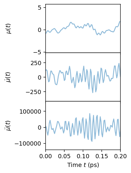
We can now read and plot the predicted dipoles. We compute the first and second time derivatives of the dipole magnitude, as the IR spectrum of the time derivatives are related to each other by factors of \(\omega\). We proceed with using the first time derivative, as that has the smoothest behavior.
[12]:
delta_t = 2e-3  # Time spacing in ps

df = DataFrame(np.loadtxt('tnep-tutorial/md/dipole.out', usecols=[1, 2, 3]), columns=['mu_x', 'mu_y', 'mu_z'])
df['time'] = df.index * delta_t
df['mu'] = np.sqrt(df.mu_x ** 2 + df.mu_y ** 2 + df.mu_z ** 2)
df.mu -= df.mu.mean()
df['dmu1'] = np.gradient(df.mu, delta_t)
df['dmu2'] = np.gradient(df.dmu1, delta_t)
[13]:
fig, axes = plt.subplots(
    figsize=(3.2, 4.2),
    dpi=140,
    nrows=3,
    sharex=True
)

axes[0].plot(df.time, df.mu, alpha=0.5)
axes[1].plot(df.time, df.dmu1, alpha=0.5)
axes[2].plot(df.time, df.dmu2, alpha=0.5)

axes[-1].set_xlabel('Time $t$ (ps)')
axes[0].set_ylabel(r'$\mu(t)$')
axes[1].set_ylabel(r'$\dot{\mu}(t)$')
axes[2].set_ylabel(r'$\ddot{\mu}(t)$')
axes[0].set_xlim(0, 0.2)

fig.tight_layout()
fig.subplots_adjust(hspace=0)
fig.align_ylabels(axes)
Finally, we compute the autocorrelation function and apply smearing in the time domain, before we Fourier transform to obtain the IR spectrum. To this end, we use functions from the dynasor package.
[14]:
from dynasor.tools.acfs import compute_acf, gaussian_decay
from dynasor.post_processing import fourier_cos_filon
THz_to_cm = 1 / 0.0299792458

t_acf, acf_mu = compute_acf(df.mu, delta_t=delta_t)
_, acf_dmu1 = compute_acf(df.dmu1, delta_t=delta_t)
_, acf_dmu2 = compute_acf(df.dmu2, delta_t=delta_t)

t_sigma = 0.1 # ps
acf_gauss = acf_dmu1 * gaussian_decay(t_acf, t_sigma=t_sigma)

# Only take first 10% of ACF
n_max = int(int(2 * len(df) * 0.1) / 2) - 1
w, S = fourier_cos_filon(acf_gauss[:n_max].reshape(1, -1), delta_t)
f = w / 2 / np.pi * THz_to_cm
ir = S.squeeze() * w  # Multiply by omega for first order derivative
[15]:
fig, axes = plt.subplots(
    figsize=(5, 4.2),
    dpi=140,
    nrows=2,
    sharex=False,
)

ax = axes[0]
ax.plot(t_acf, acf_dmu2, alpha=0.5, label='Raw ACF')
ax.plot(t_acf, acf_gauss, alpha=0.5, label='Smooth ACF')
ax.set(xlabel=r'Time $\tau$ (ps)', xlim=[0, 0.2])
ax.set_ylabel(r'$\left<\dot{\mu}(\tau)\dot{\mu}(0)\right>$')
ax.legend(loc='best', frameon=False)

ax = axes[1]
ax.plot(f, ir / np.max(ir))
ax.axhline(0, c='k', alpha=0.2)
ax.set(ylabel='IR spectrum', xlabel=r'Frequency (cm$^{-1}$)', xlim=[0, 4500])

fig.tight_layout()
fig.subplots_adjust(hspace=0.5)
fig.align_ylabels(axes)
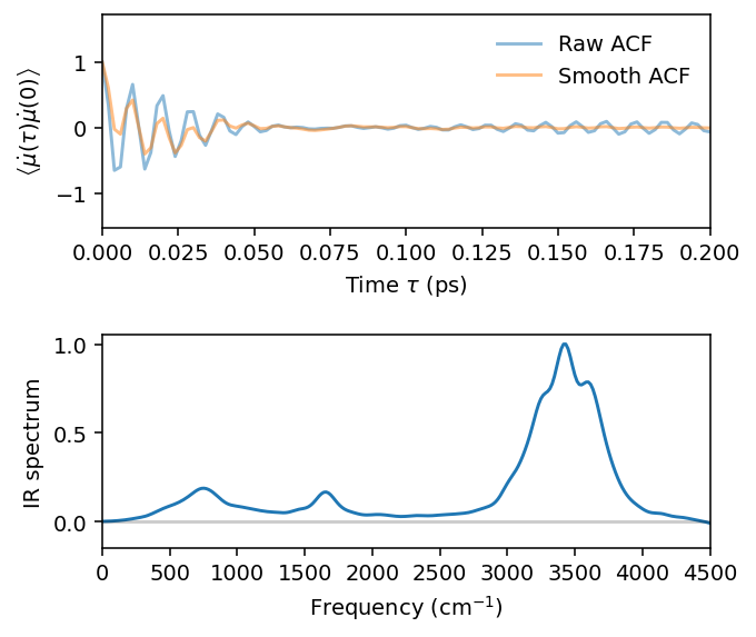
Note that this is a rough prediction of the IR spectrum. A real production simulation needs to be longer and consider a larger system to be approriately converged.